Volume Delay Functions#
Volume Delay Functions (VDFs) are mathematical functions that describe the relationship between link travel time and traffic volume. They are essential components of traffic assignment models, representing how congestion affects travel times as more vehicles use a link.
AequilibraE implements five different VDF formulations, each with distinct characteristics that make them suitable for different modeling traditions.
Available VDF Functions#
AequilibraE currently supports the following VDF functions:
BPR - Bureau of Public Roads (traditional)
BPR2 - Modified BPR with enhanced sensitivity after capacity
Conical - Spiess’ Conical function
INRETS - French INRETS function
Akcelik - Akcelik’s function for signalized intersections
VDF Comparison#
The following chart compares the behavior of all available VDF functions with their example values:
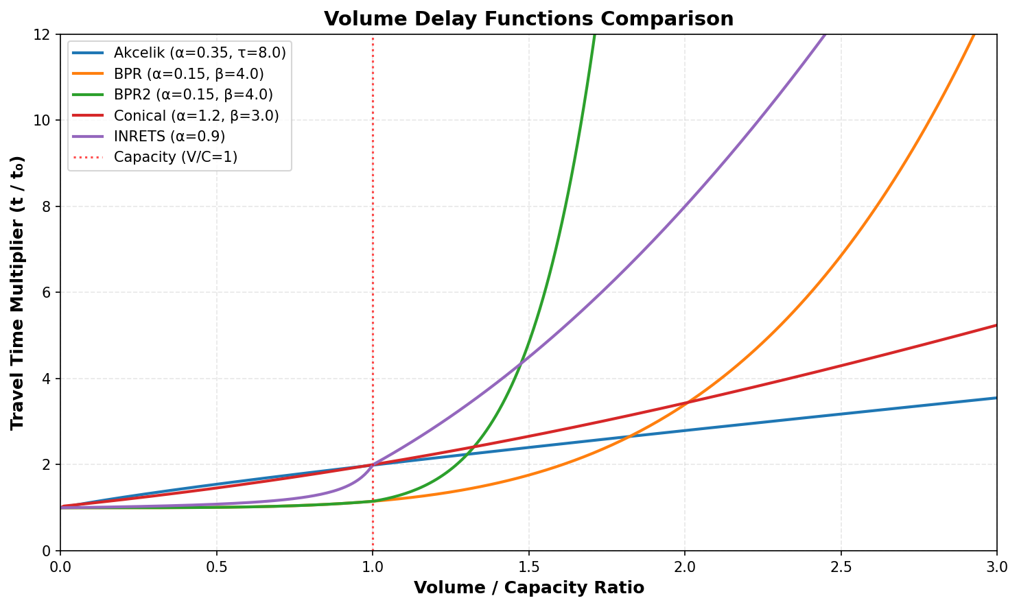
Key observations:
All functions show increasing travel times as the Volume/Capacity (V/C) ratio increases
Functions differ significantly in their behavior near and above capacity (V/C = 1)
BPR and Conical are smooth throughout the range
BPR2 and INRETS have distinct behavioral changes at capacity
Akcelik shows moderate growth rates suitable for signalized intersections
Near-Capacity Behavior#
The behavior of VDFs near capacity is particularly important for congested urban networks:
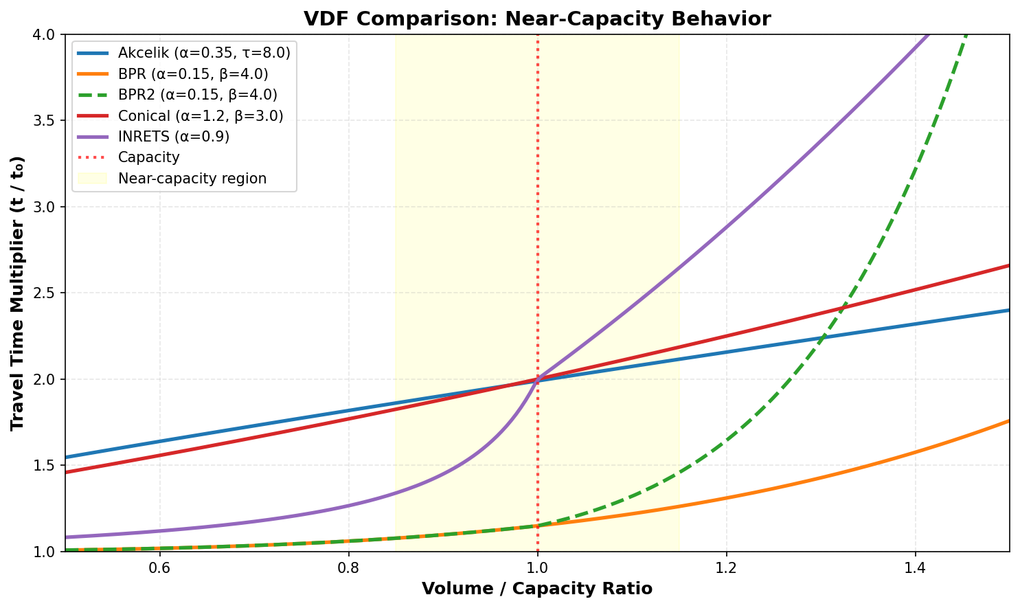
This zoomed view (V/C from 0.5 to 1.5) highlights the differences in how each function transitions from free-flow to congested conditions.
Detailed VDF Descriptions#
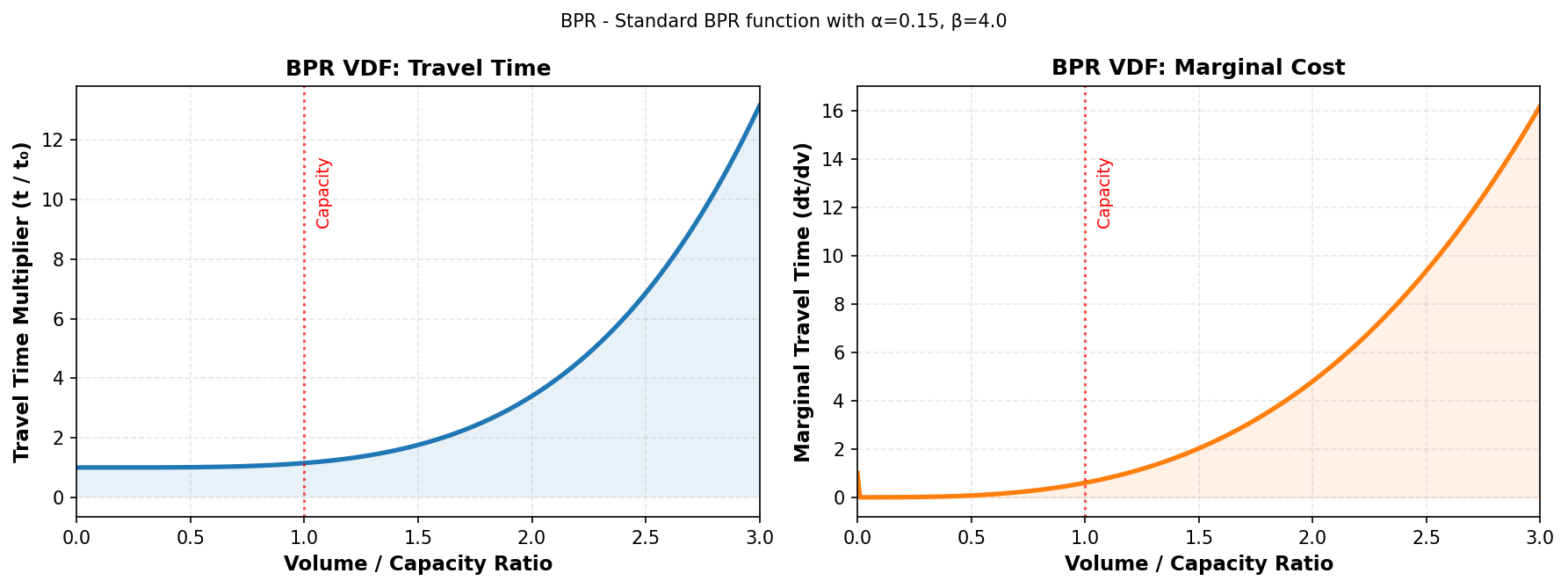
BPR (Bureau of Public Roads)#
Mathematical Formula:
- Where:
\(t\) = congested travel time
\(t_0\) = free-flow travel time
\(v\) = volume (flow) on the link
\(c\) = capacity of the link
\(\alpha\) = calibration parameter
\(\beta\) = calibration parameter (power)
- Standard Parameters:
\(\alpha = 0.15\)
\(\beta = 4.0\)
Origin and Background:
The BPR function was developed by the U.S. Bureau of Public Roads in the 1960s and has become the most widely used VDF in transportation planning. Its simplicity and effectiveness have made it the standard choice for highway assignment models worldwide.
Characteristics:
Continuous and smooth across all volume levels
Monotonically increasing (no discontinuities)
Convex function ensuring convergence in assignment algorithms
Well-suited for highway networks
Standard parameters are based on extensive empirical studies
When to Use:
Highway and freeway networks
Long-distance travel modeling
When computational stability is critical
As a baseline for comparison with other functions
When empirical data supports the standard parameters
Limitations:
May underestimate congestion effects at very high V/C ratios
Less suitable for signalized urban arterials
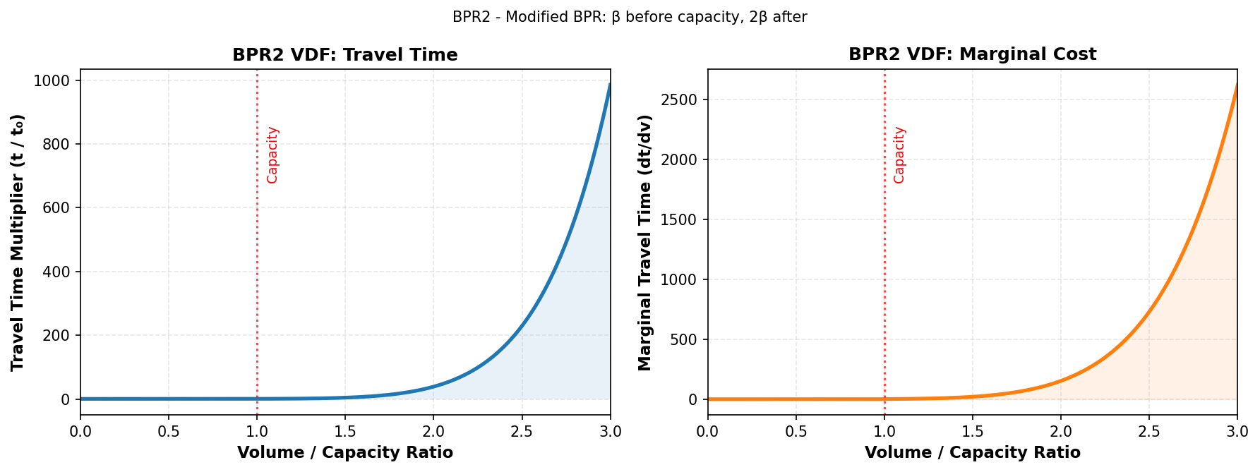
BPR2 (Modified BPR)#
Mathematical Formula:
Before capacity (\(v \leq c\)):
After capacity (\(v > c\)):
- Standard Parameters:
\(\alpha = 0.15\)
\(\beta = 4.0\)
Origin and Background:
BPR2 is a modification of the traditional BPR function designed to better represent the rapid deterioration of traffic conditions when demand exceeds capacity. The doubling of the exponent after capacity creates a steeper penalty for over-capacity conditions.
Characteristics:
Piecewise function with a transition at V/C = 1
Much steeper increase in travel time after capacity is exceeded
Maintains BPR behavior below capacity
Non-differentiable at V/C = 1 (but continuous)
More aggressive congestion penalty than standard BPR
When to Use:
Networks with strong capacity constraints
Modeling scenarios where over-capacity conditions should be heavily penalized
Mixed networks with both highways and congested urban roads
When trying to prevent unrealistic over-assignment
Limitations:
Non-differentiable point at capacity may cause convergence issues in some algorithms
The sharp transition may not reflect real-world gradual congestion buildup
Requires careful calibration of the transition behavior
Conical (Spiess)#
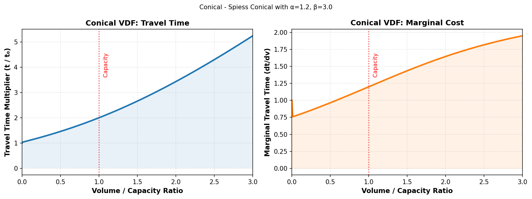
Mathematical Formula:
- Standard Parameters:
\(\alpha = 0.15\)
\(\beta = 4.0\)
Origin and Background:
Developed by Heinz Spiess in 1990, the Conical function was designed to overcome some theoretical limitations of the BPR function while maintaining computational tractability. It ensures positive derivatives everywhere and has desirable mathematical properties for convergence.
Characteristics:
Infinitely differentiable (smooth everywhere)
Asymptotic behavior as V/C approaches infinity
Guaranteed positive marginal costs
Strong theoretical foundation
Good convergence properties in equilibrium algorithms
When to Use:
When theoretical rigor is important
Transit assignment (where it was originally designed)
Networks requiring guaranteed convergence
Academic studies and benchmarking
When smooth derivatives are required throughout
Limitations:
Less intuitive parameterization than BPR
May require specialized calibration
Not as widely validated in practice as BPR
Parameters have different interpretations than BPR
INRETS (French)#
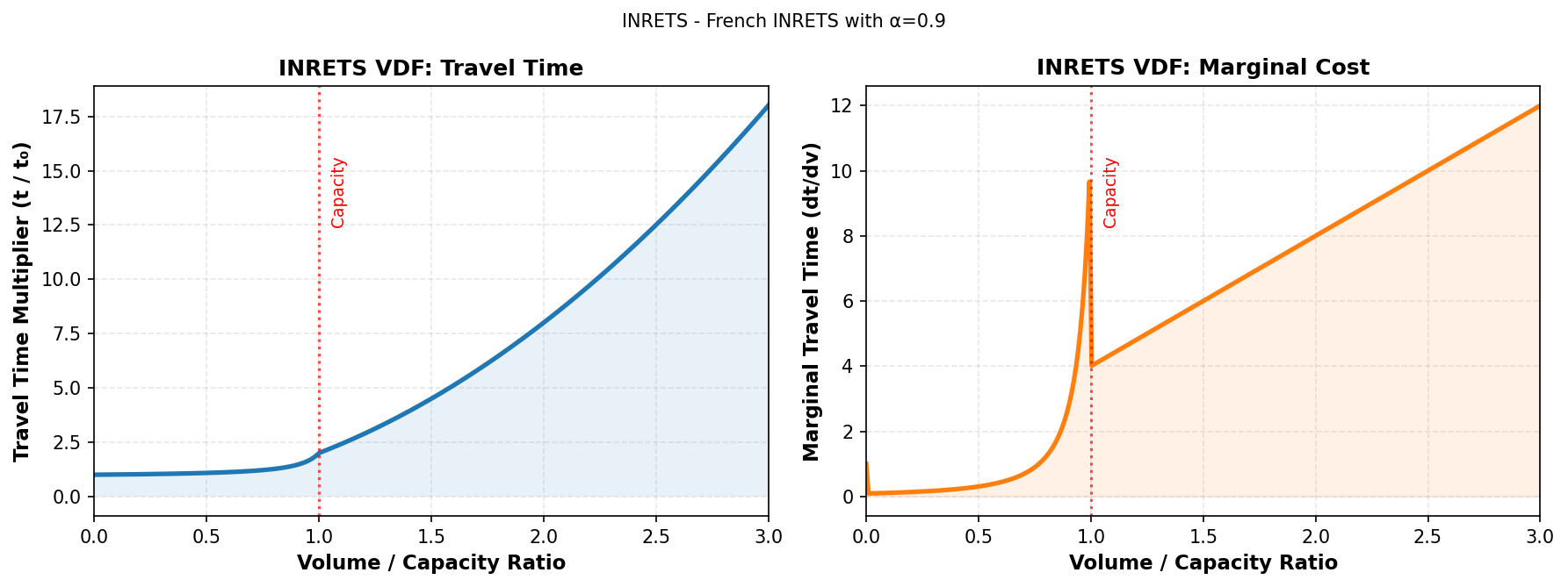
Mathematical Formula:
Before capacity (\(v \leq c\)):
After capacity (\(v > c\)):
- Standard Parameters:
\(\alpha = 1.0\) (must be \(<= 1.0\))
Origin and Background:
The INRETS function was developed by the French National Institute for Transport and Safety Research (Institut National de Recherche sur les Transports et leur Sécurité). It was designed specifically for French urban networks and reflects European traffic flow characteristics.
Characteristics:
Piecewise function with distinct before/after capacity behavior
The \(\alpha\) parameter must be less than or equal to 1.0
Hyperbolic behavior before capacity
Quadratic behavior after capacity
Designed for urban arterial roads
Reflects observed traffic patterns in French cities
When to Use:
Urban arterial networks
European-style road networks
When modeling contexts similar to French urban environments
Networks with well-defined capacity constraints
Calibrated models for specific urban areas
Limitations:
Restricted parameter range (\(\alpha <= 1.0\))
Non-differentiable at V/C = 1
Less widely used outside of Europe
May require local calibration
Dramatic change in behavior at capacity may not suit all networks
Akcelik#
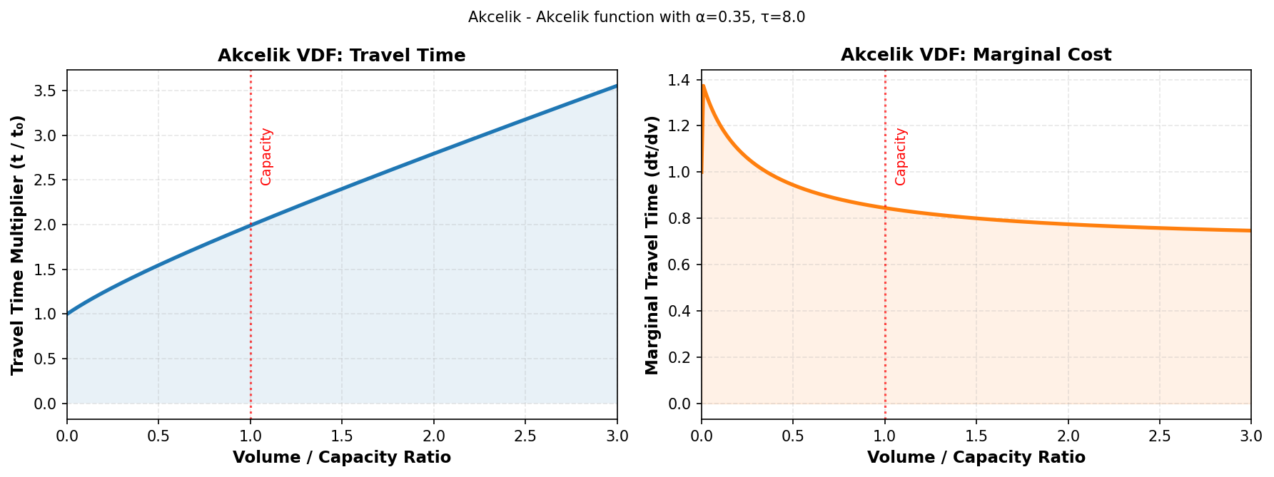
Mathematical Formula:
Where \(z = \frac{v}{c} - 1\)
- Standard Parameters:
\(\alpha = 0.25\)
\(\tau = 0.8\) (this is \(8 \times 0.1\), see note below)
Origin and Background:
Developed by Rahmi Akcelik, this function was specifically designed for signalized intersections and urban arterials. It incorporates queue theory and reflects the delay characteristics of traffic signals.
Important Note on τ Parameter:
In standard Akcelik formulations, the function includes a factor of 8 in the formula. However, in AequilibraE’s implementation, this factor of 8 has been absorbed into the \(\tau\) parameter for computational efficiency.
What this means for users:
If academic literature references a \(\tau\) value (e.g., 0.1), you must multiply it by 8 before setting it in AequilibraE
Example: To use \(\tau = 0.1\), set
tau = 0.8in AequilibraEExample: To use \(\tau = 0.15\), set
tau = 1.2in AequilibraEA value of 0.8 corresponds to a standard \(\tau = 0.1\)
Characteristics:
Specifically designed for signalized intersections
Includes queue-based delay components
Smooth transition through capacity
More moderate growth than BPR at high V/C ratios
Grounded in traffic signal theory
When to Use:
Urban networks with signalized intersections
Arterial roads with frequent signals
Australian and some Asian modeling contexts (where it’s more common)
Limitations:
Less intuitive than BPR for general highway modeling
Parameter interpretation requires understanding of signal timing
May underestimate delay on uninterrupted flow facilities
Less validated for freeway applications
Parameter Selection Guidelines#
General Recommendations#
For BPR and BPR2:
\(\alpha = 0.15\) and \(\beta = 4.0\) are widely accepted for highways
Urban arterials may benefit from \(\alpha\) values between 0.15 and 0.25
Higher \(\beta\) values (5-8) create sharper congestion curves
Lower \(\beta\) values (2-3) create more gradual curves
For Conical:
Can use similar values to BPR as starting points
\(\alpha = 0.15\) and \(\beta = 4.0\) provide comparable behavior to BPR
Fine-tuning may require understanding of the specific mathematical properties
For INRETS:
\(\alpha = 1.0\) is standard
Must satisfy \(\alpha <= 1.0\)
Higher values create steeper curves before capacity
For Akcelik:
\(\alpha = 0.25\) is typical for signalized intersections
\(\tau\) should reflect local traffic signal characteristics
Remember to use \(8 \times \tau\) in AequilibraE
Calibration Considerations#
When calibrating VDF parameters:
Use observed data: Speed-flow or travel time-volume data from your network
Consider facility types: Highways, arterials, and local streets may need different parameters
Validate results: Compare assigned volumes and speeds against counts
Test sensitivity: Understand how parameter changes affect results
Check convergence: Ensure your chosen parameters allow the algorithm to converge
Match local conditions: Standard parameters may not suit all geographic contexts
Setting VDF Parameters in AequilibraE#
In AequilibraE, VDF parameters can be set either as network-wide constants or as link-specific attributes:
Network-wide parameters:
from aequilibrae.paths import TrafficAssignment

assig = TrafficAssignment()
assig.set_vdf('BPR')
assig.set_vdf_parameters({"alpha": 0.15, "beta": 4.0})
Link-specific parameters:
# Parameters can reference field names in your network
assig.set_vdf_parameters({"alpha": "alpha_field", "beta": "beta_field"})
This flexibility allows you to:
Use different parameters for different facility types
Implement spatially varying congestion characteristics
Calibrate specific links or corridors independently
Choosing the Right VDF#
Decision Framework#
Use this decision tree to help select an appropriate VDF:
- For Highway Networks:
Start with BPR - it’s well-validated and robust
Consider BPR2 if you need stronger over-capacity penalties
Use Conical for theoretical/academic studies
- For Urban Networks:
Use Akcelik for signalized arterial networks
Consider INRETS for European-style urban contexts
BPR works as a general fallback
- For Mixed Networks:
BPR or BPR2 provide good general performance
Consider using link-specific parameters to vary behavior by facility type
- For Transit Assignment:
Conical was originally designed for transit applications
Computational Considerations#
BPR and Akcelik: Smooth everywhere, excellent convergence
Conical: Best mathematical properties, guaranteed convergence
BPR2 and INRETS: Non-differentiable at capacity, may need more iterations
All functions are computationally efficient in AequilibraE
Performance Comparison#
While individual network characteristics vary, general patterns include:
BPR: Most widely validated, good general performance
BPR2: Better for preventing unrealistic over-capacity assignment
Conical: Excellent convergence behavior, less intuitive calibration
INRETS: Good for specific urban contexts, may need local calibration
Akcelik: Best for signalized urban networks
Examples#
Basic Usage#
from aequilibrae.paths import TrafficAssignment, TrafficClass, VDF

# Check available VDF functions
vdf = VDF()
print(vdf.functions_available())
# Output: ['bpr', 'bpr2', 'conical', 'inrets', 'akcelik']

# Setup traffic assignment with BPR
assig = TrafficAssignment()
assig.set_vdf('BPR')
assig.set_vdf_parameters({"alpha": 0.15, "beta": 4.0})
Using Different VDFs#
# Highway network - standard BPR
assig.set_vdf('BPR')
assig.set_vdf_parameters({"alpha": 0.15, "beta": 4.0})

# Urban network with signals - Akcelik
assig.set_vdf('AKCELIK')
assig.set_vdf_parameters({"alpha": 0.25, "tau": 0.8})

# Network with strong capacity constraints - BPR2
assig.set_vdf('BPR2')
assig.set_vdf_parameters({"alpha": 0.15, "beta": 4.0})
Link-Specific Parameters#
# Assume your network has fields 'alpha_field' and 'beta_field'
# with values calibrated for each link
assig.set_vdf('BPR')
assig.set_vdf_parameters({"alpha": "alpha_field", "beta": "beta_field"})
References and Further Reading#
BPR Function:
Bureau of Public Roads (1964). Traffic Assignment Manual. U.S. Department of Commerce.
Conical Function:
Spiess, H. (1990). “Technical Note—Conical Volume-Delay Functions.” Transportation Science, 24(2): 153-158. https://doi.org/10.1287/trsc.24.2.153
Hampton Roads Transportation Planning Organization (2020). Regional Travel Demand Model V2 Methodology Report. Available: https://www.hrtpo.org/uploads/docs/2020_HamptonRoads_Modelv2_MethodologyReport.pdf (accessed February 2026)
Akcelik Function:
Akcelik, R. (1991). “Travel Time Functions for Transport Planning Purposes: Davidson’s Function, Its Time Dependent Form and an Alternative Travel Time Function.” Australian Road Research, 21(3): 49-59.
General Traffic Assignment:
Sheffi, Y. (1985). Urban Transportation Networks: Equilibrium Analysis with Mathematical Programming Methods. Prentice-Hall, Englewood Cliffs, NJ.
Patriksson, M. (1994). The Traffic Assignment Problem: Models and Methods. VSP, Utrecht.
Multi-class Assignment:
Zill, J., Camargo, P., Veitch, T., Daisy, N. (2019). “Toll Choice and Stochastic User Equilibrium: Ticking All the Boxes.” Transportation Research Record, 2673(4): 930-940. https://doi.org/10.1177/0361198119837496