Note
Go to the end to download the full example code.
Forecasting#
In this example, we present a full forecasting workflow for the Sioux Falls example model.
# Imports
from uuid import uuid4
from tempfile import gettempdir
from os.path import join
from aequilibrae.utils.create_example import create_example
import logging
import sys
We create the example project inside our temp folder
fldr = join(gettempdir(), uuid4().hex)

project = create_example(fldr)
logger = project.logger
Traffic assignment with skimming#
from aequilibrae.paths import TrafficAssignment, TrafficClass
We build all graphs
project.network.build_graphs()
# We get warnings that several fields in the project are filled with NaNs.
# This is true, but we won't use those fields
/opt/hostedtoolcache/Python/3.10.14/x64/lib/python3.10/site-packages/aequilibrae/project/network/network.py:327: FutureWarning: Downcasting object dtype arrays on .fillna, .ffill, .bfill is deprecated and will change in a future version. Call result.infer_objects(copy=False) instead. To opt-in to the future behavior, set `pd.set_option('future.no_silent_downcasting', True)`
  df = pd.read_sql(sql, conn).fillna(value=np.nan)
We grab the graph for cars
graph = project.network.graphs["c"]

# Let's say we want to minimize the free_flow_time
graph.set_graph("free_flow_time")

# And will skim time and distance while we are at it
graph.set_skimming(["free_flow_time", "distance"])

# And we will allow paths to be computed going through other centroids/centroid connectors
# required for the Sioux Falls network, as all nodes are centroids
graph.set_blocked_centroid_flows(False)
We get the demand matrix directly from the project record. So let’s inspect what we have in the project
proj_matrices = project.matrices
print(proj_matrices.list())
         name      file_name  ...                           description status
0  demand_omx     demand.omx  ...  Original data imported to OMX format
1   demand_mc  demand_mc.omx  ...                                  None
2       skims      skims.omx  ...                          Example skim
3  demand_aem     demand.aem  ...  Original data imported to AEM format

[4 rows x 8 columns]
Let’s get it in this better way
demand = proj_matrices.get_matrix("demand_omx")
demand.computational_view(["matrix"])
assig = TrafficAssignment()

# Create the assignment class
assigclass = TrafficClass(name="car", graph=graph, matrix=demand)

# The first thing to do is to add at list of traffic classes to be assigned
assig.add_class(assigclass)

# We set these parameters only after adding one class to the assignment
assig.set_vdf("BPR")  # This is not case-sensitive

# Then we set the volume delay function
assig.set_vdf_parameters({"alpha": "b", "beta": "power"})  # And its parameters

assig.set_capacity_field("capacity")  # The capacity and free flow travel times as they exist in the graph
assig.set_time_field("free_flow_time")

# And the algorithm we want to use to assign
assig.set_algorithm("bfw")

# Since I haven't checked the parameters file, let's make sure convergence criteria is good
assig.max_iter = 1000
assig.rgap_target = 0.001

assig.execute()  # we then execute the assignment
Convergence report is easy to see
import pandas as pd
convergence_report = assig.report()
print(convergence_report.head())
   iteration      rgap     alpha warnings     beta0     beta1  beta2
0          1       inf  1.000000           1.000000  0.000000    0.0
1          2  0.855075  0.328400           1.000000  0.000000    0.0
2          3  0.476346  0.186602           1.000000  0.000000    0.0
3          4  0.235513  0.241148           1.000000  0.000000    0.0
4          5  0.109241  0.818547           0.607382  0.392618    0.0
volumes = assig.results()
print(volumes.head())
           matrix_ab  matrix_ba   matrix_tot  ...       PCE_AB  PCE_BA      PCE_tot
link_id                                       ...
1        4502.545113        NaN  4502.545113  ...  4502.545113     NaN  4502.545113
2        8222.240524        NaN  8222.240524  ...  8222.240524     NaN  8222.240524
3        4622.925028        NaN  4622.925028  ...  4622.925028     NaN  4622.925028
4        5897.692905        NaN  5897.692905  ...  5897.692905     NaN  5897.692905
5        8101.860609        NaN  8101.860609  ...  8101.860609     NaN  8101.860609

[5 rows x 18 columns]
We could export it to CSV or AequilibraE data, but let’s put it directly into the results database
assig.save_results("base_year_assignment")
And save the skims
assig.save_skims("base_year_assignment_skims", which_ones="all", format="omx")
Trip distribution#
Calibration#
We will calibrate synthetic gravity models using the skims for TIME that we just generated
import numpy as np
from aequilibrae.distribution import GravityCalibration
Let’s take another look at what we have in terms of matrices in the model
print(proj_matrices.list())
                             name  ... status
0                      demand_omx  ...
1                       demand_mc  ...
2                           skims  ...
3                      demand_aem  ...
4  base_year_assignment_skims_car  ...

[5 rows x 8 columns]
We need the demand
demand = proj_matrices.get_matrix("demand_aem")
And the skims
imped = proj_matrices.get_matrix("base_year_assignment_skims_car")
We can check which matrix cores were created for our skims to decide which one to use
imped.names
['distance_blended', 'distance_final', 'free_flow_time_blended', 'free_flow_time_final']
Where free_flow_time_final is actually the congested time for the last iteration
But before using the data, let’s get some impedance for the intrazonals. Let’s assume it is 75% of the closest zone.
imped_core = "free_flow_time_final"
imped.computational_view([imped_core])

# If we run the code below more than once, we will be overwriting the diagonal values with non-sensical data
# so let's zero it first
np.fill_diagonal(imped.matrix_view, 0)

# We compute it with a little bit of NumPy magic
intrazonals = np.amin(imped.matrix_view, where=imped.matrix_view > 0, initial=imped.matrix_view.max(), axis=1)
intrazonals *= 0.75

# Then we fill in the impedance matrix
np.fill_diagonal(imped.matrix_view, intrazonals)
Since we are working with an OMX file, we cannot overwrite a matrix on disk So we give a new name to save it
imped.save(names=["final_time_with_intrazonals"])
This also updates these new matrices as those being used for computation as one can verify below
imped.view_names
['final_time_with_intrazonals']
We set the matrices for being used in computation
demand.computational_view(["matrix"])
for function in ["power", "expo"]:
    gc = GravityCalibration(matrix=demand, impedance=imped, function=function, nan_as_zero=True)
    gc.calibrate()
    model = gc.model
    # We save the model
    model.save(join(fldr, f"{function}_model.mod"))

    # We can save the result of applying the model as well
    # We can also save the calibration report
    with open(join(fldr, f"{function}_convergence.log"), "w") as otp:
        for r in gc.report:
            otp.write(r + "\n")
Forecast#
We create a set of ‘future’ vectors using some random growth factors. We apply the model for inverse power, as the trip frequency length distribution (TFLD) seems to be a better fit for the actual one.
from aequilibrae.distribution import Ipf, GravityApplication, SyntheticGravityModel
from aequilibrae.matrix import AequilibraeData
We compute the vectors from our matrix
origins = np.sum(demand.matrix_view, axis=1)
destinations = np.sum(demand.matrix_view, axis=0)

args = {
    "file_path": join(fldr, "synthetic_future_vector.aed"),
    "entries": demand.zones,
    "field_names": ["origins", "destinations"],
    "data_types": [np.float64, np.float64],
    "memory_mode": False,
}

vectors = AequilibraeData()
vectors.create_empty(**args)

vectors.index[:] = demand.index[:]

# Then grow them with some random growth between 0 and 10%, and balance them
vectors.origins[:] = origins * (1 + np.random.rand(vectors.entries) / 10)
vectors.destinations[:] = destinations * (1 + np.random.rand(vectors.entries) / 10)
vectors.destinations *= vectors.origins.sum() / vectors.destinations.sum()
Impedance#
imped = proj_matrices.get_matrix("base_year_assignment_skims_car")
imped.computational_view(["final_time_with_intrazonals"])
If we wanted the main diagonal to not be considered…
# np.fill_diagonal(imped.matrix_view, np.nan)
for function in ["power", "expo"]:
    model = SyntheticGravityModel()
    model.load(join(fldr, f"{function}_model.mod"))

    outmatrix = join(proj_matrices.fldr, f"demand_{function}_model.aem")
    args = {
        "impedance": imped,
        "rows": vectors,
        "row_field": "origins",
        "model": model,
        "columns": vectors,
        "column_field": "destinations",
        "nan_as_zero": True,
    }

    gravity = GravityApplication(**args)
    gravity.apply()

    # We get the output matrix and save it to OMX too,
    gravity.save_to_project(name=f"demand_{function}_modeled", file_name=f"demand_{function}_modeled.omx")
We update the matrices table/records and verify that the new matrices are indeed there
proj_matrices.update_database()
print(proj_matrices.list())
                             name  ... status
0                      demand_omx  ...
1                       demand_mc  ...
2                           skims  ...
3                      demand_aem  ...
4  base_year_assignment_skims_car  ...
5            demand_power_modeled  ...
6             demand_expo_modeled  ...

[7 rows x 8 columns]
IPF for the future vectors#
args = {
    "matrix": demand,
    "rows": vectors,
    "columns": vectors,
    "column_field": "destinations",
    "row_field": "origins",
    "nan_as_zero": True,
}

ipf = Ipf(**args)
ipf.fit()

ipf.save_to_project(name="demand_ipfd", file_name="demand_ipfd.aem")
ipf.save_to_project(name="demand_ipfd_omx", file_name="demand_ipfd.omx")
<aequilibrae.project.data.matrix_record.MatrixRecord object at 0x7fa8dd5da950>
df = proj_matrices.list()
Future traffic assignment#
from aequilibrae.paths import TrafficAssignment, TrafficClass
logger.info("\n\n\n TRAFFIC ASSIGNMENT FOR FUTURE YEAR")
demand = proj_matrices.get_matrix("demand_ipfd")

# Let's see what is the core we ended up getting. It should be 'gravity'
demand.names
['matrix']
Let’s use the IPF matrix
demand.computational_view("matrix")
assig = TrafficAssignment()

# Creates the assignment class
assigclass = TrafficClass(name="car", graph=graph, matrix=demand)

# The first thing to do is to add at a list of traffic classes to be assigned
assig.add_class(assigclass)

assig.set_vdf("BPR")  # This is not case-sensitive

# Then we set the volume delay function
assig.set_vdf_parameters({"alpha": "b", "beta": "power"})  # And its parameters

assig.set_capacity_field("capacity")  # The capacity and free flow travel times as they exist in the graph
assig.set_time_field("free_flow_time")

# And the algorithm we want to use to assign
assig.set_algorithm("bfw")

# Since I haven't checked the parameters file, let's make sure convergence criteria is good
assig.max_iter = 500
assig.rgap_target = 0.00001
Optional: Select link analysis#
If we want to execute select link analysis on a particular TrafficClass, we set the links we are analyzing.
The format of the input select links is a dictionary (str: list[tuple]).
Each entry represents a separate set of selected links to compute. The str name will name the set of links.
The list[tuple] is the list of links being selected, of the form (link_id, direction), as it occurs in the Graph.
Direction can be 0, 1, -1. 0 denotes bi-directionality
For example, let’s use Select Link on two sets of links:
select_links = {
    "Leaving node 1": [(1, 1), (2, 1)],
    "Random nodes": [(3, 1), (5, 1)],
}
We call this command on the class we are analyzing with our dictionary of values
assigclass.set_select_links(select_links)

assig.execute()  # we then execute the assignment
/opt/hostedtoolcache/Python/3.10.14/x64/lib/python3.10/site-packages/aequilibrae/paths/traffic_class.py:167: UserWarning: Input string name has a space in it. Replacing with _
  warnings.warn("Input string name has a space in it. Replacing with _")
Now let us save our select link results, all we need to do is provide it with a name In addition to exporting the select link flows, it also exports the Select Link matrices in OMX format.
assig.save_select_link_results("select_link_analysis")
Say we just want to save our select link flows, we can call:
assig.save_select_link_flows("just_flows")

# Or if we just want the SL matrices:
assig.save_select_link_matrices("just_matrices")
# Internally, the save_select_link_results calls both of these methods at once.
We could export it to CSV or AequilibraE data, but let’s put it directly into the results database
assig.save_results("future_year_assignment")
And save the skims
assig.save_skims("future_year_assignment_skims", which_ones="all", format="omx")
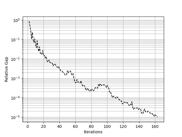
We can also plot convergence#
import matplotlib.pyplot as plt
df = assig.report()
x = df.iteration.values
y = df.rgap.values

fig = plt.figure()
ax = fig.add_subplot(111)

plt.plot(x, y, "k--")
plt.yscale("log")
plt.grid(True, which="both")
plt.xlabel(r"Iterations")
plt.ylabel(r"Relative Gap")
plt.show()
Close the project
project.close()
Total running time of the script: (0 minutes 3.465 seconds)