Hyperpath routing in the context of transit assignment

How do transit passengers choose their routes in a complex network of lines and services? How can we estimate the distribution of passenger flows and the performance of transit systems? These are some of the questions that transit assignment models aim to answer. Transit assignment models are mathematical tools that predict how passengers behave and travel in a transit network, given some assumptions and inputs.

One of the basic concepts in transit assignment models is hyperpath routing. Hyperpath routing is a way of representing the set of optimal routes that a passenger can take from an origin to a destination, based on some criterion such as travel time or generalized cost. A hyperpath is a collection of links that form a subgraph of the transit network. Each link in the hyperpath also has a probability of being used by the passenger, which reflects the attractiveness and uncertainty of the route choice. The shortest hyperpath is optimal regarding the combination of paths weighted by the probability of being used.

Hyperpath routing can be applied to different types of transit assignment models, but in this following page we will focus on frequency-based models. Frequency-based models assume that passengers do not have reliable information about the service schedules and arrival times, and they choose their routes based on the expected travel time or cost. This type of model is suitable for transit systems with rather frequent services.

To illustrate how hyperpath routing works in frequency-based models, we will use the classic algorithm by Spiess & Florian [1] implemented in AequilibraE.

We will use a simple grid network as an Python example to demonstrate how a hyperpath depends on link frequency for a given origin-destination pair. Note that it can be extended to other contexts such as risk-averse vehicle navigation [2].

Let’s start by importing some Python packages.

Imports

import matplotlib.pyplot as plt
import networkx as nx
import numpy as np
import pandas as pd
from aequilibrae.paths.public_transport import HyperpathGenerating
from numba import jit

RS = 124  # random seed
FS = (6, 6)  # figure size

Bell’s network

We start by defining the directed graph \(\mathcal{G} = \left( V, E \right)\), where \(V\) and \(E\) are the graph vertices and edges. The hyperpath generating algorithm requires 2 attributes for each edge \(a \in V\):

• edge travel time \(u_a \geq 0\)

• edge frequency \(f_a \geq 0\)

The edge frequency is inversely related to the exposure to delay. For example, in a transit network, a boarding edge has a frequency that is the inverse of the headway (or half the headway, depending on the model assumptions). A walking edge has no exposure to delay, so its frequency is assumed to be infinite.

Bell’s network is a synthetic network: it is a \(n\)-by-\(n\) grid bi-directional network [2], [3]. The edge travel time is taken as random number following a uniform distribution:

\[u_a \sim \mathbf{U}[0,1)\]

To demonstrate how the hyperpath depends on the exposure to delay, we will use a positive constant \(\alpha\) and a base delay \(d_a\) for each edge that follows a uniform distribution:

\[d_a \sim \mathbf{U}[0,1)\]

The constant \(\alpha \geq 0\) allows us to adjust the edge frequency as follows:

\[\begin{split}f_a = \left\{ \begin{array}{ll} 1 / \left( \alpha \; d_a \right) & \text{if $\alpha \; d_a \neq 0$} \\ \infty & \text{otherwise} \\ \end{array} \right.\end{split}\]

A smaller \(\alpha\) value implies higher edge frequencies, and vice versa. Next, we will create the network as a pandas dataframe.

Vertices

def create_vertices(n):
    x = np.linspace(0, 1, n)
    y = np.linspace(0, 1, n)
    xv, yv = np.meshgrid(x, y, indexing="xy")
    vertices = pd.DataFrame()
    vertices["x"] = xv.ravel()
    vertices["y"] = yv.ravel()
    return vertices

n = 10
vertices = create_vertices(n)
vertices.head(3)

	x	y
0	0.000000	0.0
1	0.111111	0.0
2	0.222222	0.0

@jit
def create_edges_numba(n):
    m = 2 * n * (n - 1)
    tail = np.zeros(m, dtype=np.uint32)
    head = np.zeros(m, dtype=np.uint32)
    k = 0
    for i in range(n - 1):
        for j in range(n):
            tail[k] = i + j * n
            head[k] = i + 1 + j * n
            k += 1
            tail[k] = j + i * n
            head[k] = j + (i + 1) * n
            k += 1
    return tail, head


def create_edges(n, seed=124):
    tail, head = create_edges_numba(n)
    edges = pd.DataFrame()
    edges["tail"] = tail
    edges["head"] = head
    m = len(edges)
    rng = np.random.default_rng(seed=seed)
    edges["trav_time"] = rng.uniform(0.0, 1.0, m)
    edges["delay_base"] = rng.uniform(0.0, 1.0, m)
    return edges

edges = create_edges(n, seed=RS)
edges.head(3)

	tail	head	trav_time	delay_base
0	0	1	0.785253	0.287917
1	0	10	0.785859	0.970429
2	10	11	0.969136	0.854512

Plot the network

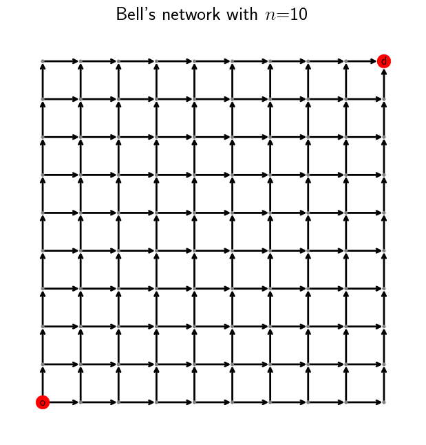
We use the NetworkX package to plot the network. The bottom left vertex is the origin (‘o’) and the top right vertex is the destination (‘d’) for the hyperpath computation.

# NetworkX
n_vertices = n * n
pos = vertices[["x", "y"]].values
G = nx.from_pandas_edgelist(
    edges,
    source="tail",
    target="head",
    edge_attr=["trav_time", "delay_base"],
    create_using=nx.DiGraph,
)
widths = 2
figure = plt.figure(figsize=FS)
node_colors = n_vertices * ["gray"]
node_colors[0] = "r"
node_colors[-1] = "r"
ns = 100 / n
node_size = n_vertices * [ns]
node_size[0] = 20 * ns
node_size[-1] = 20 * ns
labeldict = {}
labeldict[0] = "o"
labeldict[n * n - 1] = "d"
nx.draw(
    G,
    pos=pos,
    width=widths,
    node_size=node_size,
    node_color=node_colors,
    arrowstyle="->",
    labels=labeldict,
    with_labels=True,
)
ax = plt.gca()
_ = ax.set_title(f"Bell's network with $n$={n}", color="k")

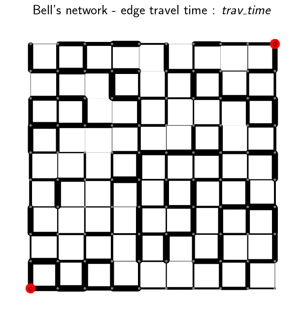
We can also visualize the edge travel time:

widths = 1e2 * np.array([G[u][v]["trav_time"] for u, v in G.edges()]) / n
_ = plt.figure(figsize=FS)
node_colors = n_vertices * ["gray"]
node_colors[0] = "r"
node_colors[-1] = "r"
ns = 100 / n
node_size = n_vertices * [ns]
node_size[0] = 20 * ns
node_size[-1] = 20 * ns
labeldict = {}
labeldict[0] = "o"
labeldict[n * n - 1] = "d"
nx.draw(
    G,
    pos=pos,
    width=widths,
    node_size=node_size,
    node_color=node_colors,
    arrowstyle="-",
    labels=labeldict,
    with_labels=True,
)
ax = plt.gca()
_ = ax.set_title(
    "Bell's network - edge travel time :  $\\textit{trav_time}$", color="k"
)

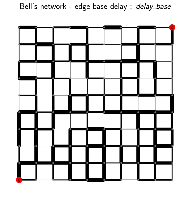
And the base delay:

widths = 1e2 * np.array([G[u][v]["delay_base"] for u, v in G.edges()]) / n
_ = plt.figure(figsize=FS)
node_colors = n_vertices * ["gray"]
node_colors[0] = "r"
node_colors[-1] = "r"
ns = 100 / n
node_size = n_vertices * [ns]
node_size[0] = 20 * ns
node_size[-1] = 20 * ns
labeldict = {}
labeldict[0] = "o"
labeldict[n * n - 1] = "d"
nx.draw(
    G,
    pos=pos,
    width=widths,
    node_size=node_size,
    node_color=node_colors,
    arrowstyle="-",
    labels=labeldict,
    with_labels=True,
)
ax = plt.gca()
_ = ax.set_title("Bell's network - edge base delay : $\\textit{delay_base}$", color="k")

Hyperpath computation

We now introduce a function plot_shortest_hyperpath that:

• creates the network,

• computes the edge frequency given an input value for \(\alpha\),

• compute the shortest hyperpath,

• plot the network and hyperpath with NetworkX.

def plot_shortest_hyperpath(n=10, alpha=10.0, figsize=FS, seed=RS):

    # network creation
    vertices = create_vertices(n)
    n_vertices = n * n
    edges = create_edges(n, seed=seed)
    delay_base = edges.delay_base.values
    indices = np.where(delay_base == 0.0)
    delay_base[indices] = 1.0
    freq_base = 1.0 / delay_base
    freq_base[indices] = np.inf
    edges["freq_base"] = freq_base
    if alpha == 0.0:
        edges["freq"] = np.inf
    else:
        edges["freq"] = edges.freq_base / alpha

    # Spiess & Florian
    sf = HyperpathGenerating(
        edges, tail="tail", head="head", trav_time="trav_time", freq="freq"
    )
    sf.run(origin=0, destination=n * n - 1, volume=1.0)

    # NetworkX
    pos = vertices[["x", "y"]].values
    G = nx.from_pandas_edgelist(
        sf._edges,
        source="tail",
        target="head",
        edge_attr="volume",
        create_using=nx.DiGraph,
    )
    widths = 1e2 * np.array([G[u][v]["volume"] for u, v in G.edges()]) / n
    figure = plt.figure(figsize=figsize)
    node_colors = n_vertices * ["gray"]
    node_colors[0] = "r"
    node_colors[-1] = "r"
    ns = 100 / n
    node_size = n_vertices * [ns]
    node_size[0] = 20 * ns
    node_size[-1] = 20 * ns
    labeldict = {}
    labeldict[0] = "o"
    labeldict[n * n - 1] = "d"
    nx.draw(
        G,
        pos=pos,
        width=widths,
        node_size=node_size,
        node_color=node_colors,
        arrowstyle="-",
        labels=labeldict,
        with_labels=True,
    )
    ax = plt.gca()
    _ = ax.set_title(
        f"Shortest hyperpath - Bell's network $\\alpha$={alpha}", color="k"
    )

We start with \(\alpha=0\). This implies that there is no delay over all the network.

plot_shortest_hyperpath(n=10, alpha=0.0)

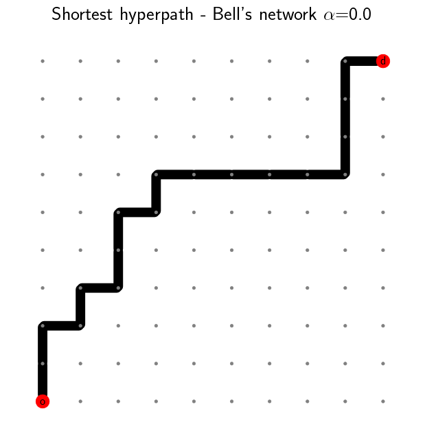
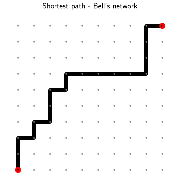
The hyperpath that we obtain is the same as the shortest path that Dijkstra’s algorithm would have computed. We call NetworkX’s dijkstra_path method in order to compute the shortest path:

G = nx.from_pandas_edgelist(
    sf._edges,
    source="tail",
    target="head",
    edge_attr="trav_time",
    create_using=nx.DiGraph,
)

# Dijkstra
nodes = nx.dijkstra_path(G, 0, n*n-1, weight='trav_time')
edges = list(nx.utils.pairwise(nodes))

# plot
figure = plt.figure(figsize=FS)
node_colors = n_vertices * ["gray"]
node_colors[0] = "r"
node_colors[-1] = "r"
ns = 100 / n
node_size = n_vertices * [ns]
node_size[0] = 20 * ns
node_size[-1] = 20 * ns
labeldict = {}
labeldict[0] = "o"
labeldict[n * n - 1] = "d"
widths = 1e2 * np.array([1 if (u,v) in edges else 0 for u, v in G.edges()]) / n
pos = vertices[["x", "y"]].values
nx.draw(
    G,
    pos=pos,
    width=widths,
    node_size=node_size,
    node_color=node_colors,
    arrowstyle="-",
    labels=labeldict,
    with_labels=True,
)
ax = plt.gca()
_ = ax.set_title(
    f"Shortest path - Bell's network", color="k"
)

Let’s introduce some delay by increasing the value of \(\alpha\):

plot_shortest_hyperpath(n=10, alpha=0.5)

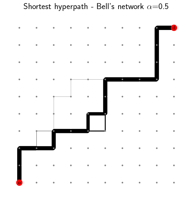
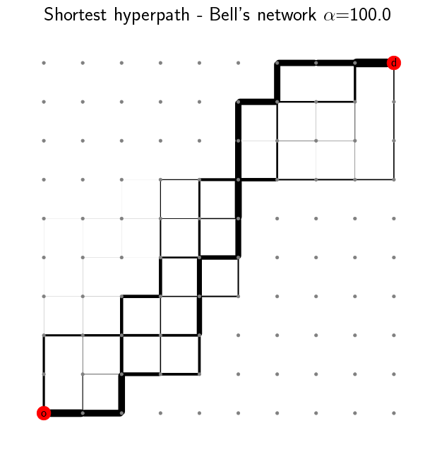
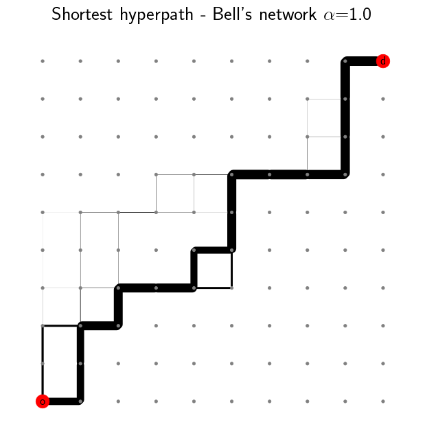
The shortest path is no longer unique and multiple routes are suggested. The link usage probability is reflected by the line width. The majority of the flow still follows the shortest path, but some of it is distributed among different alternative paths. This becomes more apparent as we further increase \(\alpha\):

plot_shortest_hyperpath(n=10, alpha=1.0)

plot_shortest_hyperpath(n=10, alpha=100.0)

References

[1]

Spiess, H., Florian, M. (1989) “Optimal strategies: A new assignment model for transit networks”. Transportation Research Part B: Methodological, 23(2), 83-102. Available in: https://doi.org/10.1016/0191-2615(89)90034-9

[2] (1,2)

Ma, J., Fukuda, D., Schmöcker, J. D. (2012) “Faster hyperpath generating algorithms for vehicle navigation”, Transportmetrica A: Transport Science, 9(10), 925–948. Available in: https://doi.org/10.1080/18128602.2012.719165

[3]

Bell, M. G. H. (2009) “Hyperstar: A multi-path Astar algorithm for risk averse vehicle navigation”, Transportation Research Part B: Methodological, 43(1), 97-107. Available in: https://doi.org/10.1016/j.trb.2008.05.010.