Note
Click here to download the full example code
7.15. Forecasting
On this example we present a full forecasting workflow for the Sioux Falls example model.
## Imports
from uuid import uuid4
from tempfile import gettempdir
from os.path import join
from aequilibrae.utils.create_example import create_example
import logging
import sys
We create the example project inside our temp folder
fldr = join(gettempdir(), uuid4().hex)

project = create_example(fldr)
logger = project.logger

# We the project open, we can tell the logger to direct all messages to the terminal as well
stdout_handler = logging.StreamHandler(sys.stdout)
formatter = logging.Formatter("%(asctime)s;%(levelname)s ; %(message)s")
stdout_handler.setFormatter(formatter)
logger.addHandler(stdout_handler)
## Traffic assignment with skimming
from aequilibrae.paths import TrafficAssignment, TrafficClass
# we build all graphs
project.network.build_graphs()
# We get warnings that several fields in the project are filled with NaNs.  Which is true, but we won't use those fields
2023-01-16 13:35:25,625;WARNING ; Field(s) name, lanes has(ve) at least one NaN value. Check your computations
2023-01-16 13:35:25,658;WARNING ; Field(s) name, lanes has(ve) at least one NaN value. Check your computations
2023-01-16 13:35:25,691;WARNING ; Field(s) name, lanes has(ve) at least one NaN value. Check your computations
2023-01-16 13:35:25,724;WARNING ; Field(s) name, lanes has(ve) at least one NaN value. Check your computations
2023-01-16 13:35:25,757;WARNING ; Field(s) name, lanes has(ve) at least one NaN value. Check your computations
2023-01-16 13:35:25,789;WARNING ; Field(s) name, lanes has(ve) at least one NaN value. Check your computations
# we grab the graph for cars
graph = project.network.graphs["c"]

# let's say we want to minimize free_flow_time
graph.set_graph("free_flow_time")

# And will skim time and distance while we are at it
graph.set_skimming(["free_flow_time", "distance"])

# And we will allow paths to be compute going through other centroids/centroid connectors
# required for the Sioux Falls network, as all nodes are centroids
graph.set_blocked_centroid_flows(False)
/home/runner/work/aequilibrae/aequilibrae/aequilibrae/paths/graph.py:445: FutureWarning: The default value of numeric_only in DataFrameGroupBy.sum is deprecated. In a future version, numeric_only will default to False. Either specify numeric_only or select only columns which should be valid for the function.
  df = self.__graph_groupby.sum()[[cost_field]].reset_index()
2023-01-16 13:35:25,815;WARNING ; Cost field with wrong type. Converting to float64
/home/runner/work/aequilibrae/aequilibrae/aequilibrae/paths/graph.py:479: FutureWarning: The default value of numeric_only in DataFrameGroupBy.sum is deprecated. In a future version, numeric_only will default to False. Either specify numeric_only or select only columns which should be valid for the function.
  df = self.__graph_groupby.sum()[skim_fields].reset_index()
# We get the demand matrix directly from the project record
# so let's inspect what we have in the project
proj_matrices = project.matrices
proj_matrices.list()
# Let's get it in this better way
demand = proj_matrices.get_matrix("demand_omx")
demand.computational_view(["matrix"])
assig = TrafficAssignment()

# Creates the assignment class
assigclass = TrafficClass(name="car", graph=graph, matrix=demand)

# The first thing to do is to add at list of traffic classes to be assigned
assig.add_class(assigclass)

# We set these parameters only after adding one class to the assignment
assig.set_vdf("BPR")  # This is not case-sensitive # Then we set the volume delay function

assig.set_vdf_parameters({"alpha": "b", "beta": "power"})  # And its parameters

assig.set_capacity_field("capacity")  # The capacity and free flow travel times as they exist in the graph
assig.set_time_field("free_flow_time")

# And the algorithm we want to use to assign
assig.set_algorithm("bfw")

# since I haven't checked the parameters file, let's make sure convergence criteria is good
assig.max_iter = 1000
assig.rgap_target = 0.001

assig.execute()  # we then execute the assignment
/home/runner/work/aequilibrae/aequilibrae/aequilibrae/paths/graph.py:445: FutureWarning: The default value of numeric_only in DataFrameGroupBy.sum is deprecated. In a future version, numeric_only will default to False. Either specify numeric_only or select only columns which should be valid for the function.
  df = self.__graph_groupby.sum()[[cost_field]].reset_index()
2023-01-16 13:35:26,081;WARNING ; Cost field with wrong type. Converting to float64
2023-01-16 13:35:26,081;INFO ; bfw Assignment STATS
2023-01-16 13:35:26,081;INFO ; Iteration, RelativeGap, stepsize
2023-01-16 13:35:26,088;INFO ; 1,inf,1.0
2023-01-16 13:35:26,093;INFO ; 2,0.8550751349428284,0.32839952448634563
2023-01-16 13:35:26,101;INFO ; 3,0.4763455007221067,0.18660240547488702
2023-01-16 13:35:26,107;INFO ; 4,0.2355126365951965,0.2411477440291793
2023-01-16 13:35:26,115;INFO ; 5,0.10924072010481088,0.8185470737942447
2023-01-16 13:35:26,121;INFO ; 6,0.1980945227617506,0.14054330572978305
2023-01-16 13:35:26,127;INFO ; 7,0.0668172221544687,0.36171152718899247
2023-01-16 13:35:26,132;INFO ; 8,0.06792122267870587,0.9634685345644044
2023-01-16 13:35:26,137;INFO ; 9,0.10705582933092855,0.13757153109677187
2023-01-16 13:35:26,142;INFO ; 10,0.04038814432034622,0.1609403425427973
2023-01-16 13:35:26,147;INFO ; 11,0.025801226183773084,0.716435057617116
2023-01-16 13:35:26,153;INFO ; 12,0.042846437173170424,0.08581544277016687
2023-01-16 13:35:26,162;INFO ; 13,0.016971662333407043,0.1660157969033195
2023-01-16 13:35:26,167;INFO ; 14,0.020396548012132195,0.4461322062863191
2023-01-16 13:35:26,172;INFO ; 15,0.025887901335905694,0.08515995223661561
2023-01-16 13:35:26,177;INFO ; 16,0.015188959427663162,0.1988698342670051
2023-01-16 13:35:26,182;INFO ; 17,0.01475141964322897,0.3548856159715819
2023-01-16 13:35:26,187;INFO ; 18,0.015582407302127808,0.06145415154081679
2023-01-16 13:35:26,193;INFO ; 19,0.008935871473338547,0.08603462968532699
2023-01-16 13:35:26,198;INFO ; 20,0.008477045208211683,0.1668913886047936
2023-01-16 13:35:26,203;INFO ; 21,0.009517581409988221,0.4917099156011133
2023-01-16 13:35:26,209;INFO ; 22,0.013060711845093087,0.060284308755231206
2023-01-16 13:35:26,214;INFO ; 23,0.006861821876765184,0.10954009782378307
2023-01-16 13:35:26,219;INFO ; 24,0.006201113315688483,0.12230718464290123
2023-01-16 13:35:26,224;INFO ; 25,0.0074574049738041406,0.3080614235512652
2023-01-16 13:35:26,230;INFO ; 26,0.006900497787039256,0.32835666337221175
2023-01-16 13:35:26,234;INFO ; 27,0.006963554132391016,0.7377893941135681
2023-01-16 13:35:26,239;INFO ; 28,0.006817764279834173,0.0443870768699142
2023-01-16 13:35:26,244;INFO ; 29,0.004277860366532555,0.05431813621783447
2023-01-16 13:35:26,250;INFO ; 30,0.004136181096381436,0.05758294976347482
2023-01-16 13:35:26,254;INFO ; 31,0.0031483923250298237,0.0918038853550363
2023-01-16 13:35:26,259;INFO ; 32,0.0034184967969881734,0.12279944254979965
2023-01-16 13:35:26,264;INFO ; 33,0.002738614050254322,0.08799214942487946
2023-01-16 13:35:26,270;INFO ; 34,0.0023403784016331874,0.1098259985006849
2023-01-16 13:35:26,275;INFO ; 35,0.0023185435502055523,0.18741920884713098
2023-01-16 13:35:26,280;INFO ; 36,0.0023838181828793143,0.1404967362503087
2023-01-16 13:35:26,285;INFO ; 37,0.0017801377860521138,0.25278698153070905
2023-01-16 13:35:26,290;INFO ; 38,0.0019264349761422953,0.30768123024764726
2023-01-16 13:35:26,295;INFO ; 39,0.0018408894375062524,0.3982324050247662
2023-01-16 13:35:26,300;INFO ; 40,0.0018205742523357215,0.5255149131180074
2023-01-16 13:35:26,306;INFO ; 41,0.0020224171108353135,0.012343794696331265
2023-01-16 13:35:26,311;INFO ; 42,0.001423836778473865,0.03045402621736974
2023-01-16 13:35:26,316;INFO ; 43,0.0011877471305860427,0.02283308748607117
2023-01-16 13:35:26,321;INFO ; 44,0.0012106681494599195,0.06969126002892805
2023-01-16 13:35:26,325;INFO ; 45,0.0011336232568064097,0.038970964685986896
2023-01-16 13:35:26,330;INFO ; 46,0.0009780989052684459,0.022071990851560294
2023-01-16 13:35:26,330;INFO ; bfw Assignment finished. 46 iterations and 0.0009780989052684459 final gap
# Convergence report is easy to see
import pandas as pd

convergence_report = assig.report()
convergence_report.head()
volumes = assig.results()
volumes.head()
# We could export it to CSV or AequilibraE data, but let's put it directly into the results database
assig.save_results("base_year_assignment")
# And save the skims
assig.save_skims("base_year_assignment_skims", which_ones="all", format="omx")
2023-01-16 13:35:26,384;WARNING ; Matrix Record has been saved to the database
## Trip distribution
### Calibration
# We will calibrate synthetic gravity models using the skims for TIME that we just generated
import numpy as np
from aequilibrae.distribution import GravityCalibration
# Let's take another look at what we have in terms of matrices in the model
proj_matrices.list()
# We need the demand
demand = proj_matrices.get_matrix("demand_aem")

# And the skims
imped = proj_matrices.get_matrix("base_year_assignment_skims_car")
# We can check which matrix cores were created for our skims to decide which one to use
imped.names

# Where free_flow_time_final is actually the congested time for the last iteration
['distance_blended', 'distance_final', 'free_flow_time_blended', 'free_flow_time_final']
# But before using the data, let's get some impedance for the intrazonals
# Let's assume it is 75% of the closest zone
imped_core = "free_flow_time_final"
imped.computational_view([imped_core])

# If we run the code below more than once, we will be overwriting the diagonal values with non-sensical data
# so let's zero it first
np.fill_diagonal(imped.matrix_view, 0)

# We compute it with a little bit of NumPy magic
intrazonals = np.amin(imped.matrix_view, where=imped.matrix_view > 0, initial=imped.matrix_view.max(), axis=1)
intrazonals *= 0.75

# Then we fill in the impedance matrix
np.fill_diagonal(imped.matrix_view, intrazonals)
# Since we are working with an OMX file, we cannot overwrite a matrix on disk
# So we give a new name to save it
imped.save(names=["final_time_with_intrazonals"])
# This also updates these new matrices as those being used for computation
# As one can verify below
imped.view_names
['final_time_with_intrazonals']
# We set the matrices for being used in computation
demand.computational_view(["matrix"])
for function in ["power", "expo"]:
    gc = GravityCalibration(matrix=demand, impedance=imped, function=function, nan_as_zero=True)
    gc.calibrate()
    model = gc.model
    # we save the model
    model.save(join(fldr, f"{function}_model.mod"))

    # We can save the result of applying the model as well
    # we can also save the calibration report
    with open(join(fldr, f"{function}_convergence.log"), "w") as otp:
        for r in gc.report:
            otp.write(r + "\n")
## Forecast
#  * We create a set of * 'future' * vectors using some random growth factors
#  * We apply the model for inverse power, as the TFLD seems to be a better fit for the actual one
from aequilibrae.distribution import Ipf, GravityApplication, SyntheticGravityModel
from aequilibrae.matrix import AequilibraeData
import numpy as np
# We compute the vectors from our matrix
origins = np.sum(demand.matrix_view, axis=1)
destinations = np.sum(demand.matrix_view, axis=0)

args = {
    "file_path": join(fldr, "synthetic_future_vector.aed"),
    "entries": demand.zones,
    "field_names": ["origins", "destinations"],
    "data_types": [np.float64, np.float64],
    "memory_mode": False,
}

vectors = AequilibraeData()
vectors.create_empty(**args)

vectors.index[:] = demand.index[:]

# Then grow them with some random growth between 0 and 10% - Plus balance them
vectors.origins[:] = origins * (1 + np.random.rand(vectors.entries) / 10)
vectors.destinations[:] = destinations * (1 + np.random.rand(vectors.entries) / 10)
vectors.destinations *= vectors.origins.sum() / vectors.destinations.sum()
# Impedance
imped = proj_matrices.get_matrix("base_year_assignment_skims_car")
imped.computational_view(["final_time_with_intrazonals"])

# If we wanted the main diagonal to not be considered...
# np.fill_diagonal(imped.matrix_view, np.nan)
for function in ["power", "expo"]:
    model = SyntheticGravityModel()
    model.load(join(fldr, f"{function}_model.mod"))

    outmatrix = join(proj_matrices.fldr, f"demand_{function}_model.aem")
    apply = GravityApplication()
    args = {
        "impedance": imped,
        "rows": vectors,
        "row_field": "origins",
        "model": model,
        "columns": vectors,
        "column_field": "destinations",
        "nan_as_zero": True,
    }

    gravity = GravityApplication(**args)
    gravity.apply()

    # We get the output matrix and save it to OMX too,
    gravity.save_to_project(name=f"demand_{function}_modeled", file_name=f"demand_{function}_modeled.omx")
2023-01-16 13:35:27,108;WARNING ; Matrix Record has been saved to the database
2023-01-16 13:35:27,230;WARNING ; Matrix Record has been saved to the database
# We update the matrices table/records and verify that the new matrices are indeed there
proj_matrices.update_database()
proj_matrices.list()
### We now run IPF for the future vectors
args = {
    "matrix": demand,
    "rows": vectors,
    "columns": vectors,
    "column_field": "destinations",
    "row_field": "origins",
    "nan_as_zero": True,
}

ipf = Ipf(**args)
ipf.fit()

ipf.save_to_project(name="demand_ipfd", file_name="demand_ipfd.aem")
ipf.save_to_project(name="demand_ipfd_omx", file_name="demand_ipfd.omx")
2023-01-16 13:35:27,285;WARNING ; Matrix Record has been saved to the database
2023-01-16 13:35:27,298;WARNING ; Matrix Record has been saved to the database

<aequilibrae.project.data.matrix_record.MatrixRecord object at 0x7f51c0d41b20>
proj_matrices.list()
## Future traffic assignment
from aequilibrae.paths import TrafficAssignment, TrafficClass
logger.info("\n\n\n TRAFFIC ASSIGNMENT FOR FUTURE YEAR")
2023-01-16 13:35:27,308;INFO ;


 TRAFFIC ASSIGNMENT FOR FUTURE YEAR
demand = proj_matrices.get_matrix("demand_ipfd")

# let's see what is the core we ended up getting. It should be 'gravity'
demand.names
['matrix']
# Let's use the IPF matrix
demand.computational_view("matrix")

assig = TrafficAssignment()

# Creates the assignment class
assigclass = TrafficClass(name="car", graph=graph, matrix=demand)

# The first thing to do is to add at list of traffic classes to be assigned
assig.add_class(assigclass)

assig.set_vdf("BPR")  # This is not case-sensitive # Then we set the volume delay function

assig.set_vdf_parameters({"alpha": "b", "beta": "power"})  # And its parameters

assig.set_capacity_field("capacity")  # The capacity and free flow travel times as they exist in the graph
assig.set_time_field("free_flow_time")

# And the algorithm we want to use to assign
assig.set_algorithm("bfw")

# since I haven't checked the parameters file, let's make sure convergence criteria is good
assig.max_iter = 500
assig.rgap_target = 0.00001

assig.execute()  # we then execute the assignment
/home/runner/work/aequilibrae/aequilibrae/aequilibrae/paths/graph.py:445: FutureWarning: The default value of numeric_only in DataFrameGroupBy.sum is deprecated. In a future version, numeric_only will default to False. Either specify numeric_only or select only columns which should be valid for the function.
  df = self.__graph_groupby.sum()[[cost_field]].reset_index()
2023-01-16 13:35:27,564;WARNING ; Cost field with wrong type. Converting to float64
2023-01-16 13:35:27,564;INFO ; bfw Assignment STATS
2023-01-16 13:35:27,564;INFO ; Iteration, RelativeGap, stepsize
2023-01-16 13:35:27,571;INFO ; 1,inf,1.0
2023-01-16 13:35:27,579;INFO ; 2,0.8780283220741393,0.3191095155781166
2023-01-16 13:35:27,587;INFO ; 3,0.5302378283465513,0.16229273552620688
2023-01-16 13:35:27,595;INFO ; 4,0.29541230746848735,0.19208769334500417
2023-01-16 13:35:27,603;INFO ; 5,0.09233118279988412,0.7601907450429835
2023-01-16 13:35:27,612;INFO ; 6,0.27370627510530143,0.11097037967912722
2023-01-16 13:35:27,618;INFO ; 7,0.10317211601901224,0.2210327675036471
2023-01-16 13:35:27,624;INFO ; 8,0.06505966184142942,0.711193234954081
2023-01-16 13:35:27,634;INFO ; 9,0.10668143387123219,0.13311802651469315
2023-01-16 13:35:27,641;INFO ; 10,0.047003226080616016,0.18656706260961176
2023-01-16 13:35:27,647;INFO ; 11,0.02980528824382008,0.7620819044190782
2023-01-16 13:35:27,655;INFO ; 12,0.06347445943212231,0.08479774378777985
2023-01-16 13:35:27,661;INFO ; 13,0.02157259882995468,0.22025433506635686
2023-01-16 13:35:27,669;INFO ; 14,0.03105441268622069,0.08394404829939456
2023-01-16 13:35:27,676;INFO ; 15,0.013967751061782017,0.26164310694821846
2023-01-16 13:35:27,682;INFO ; 16,0.024396334241515556,0.08353230675594439
2023-01-16 13:35:27,688;INFO ; 17,0.010929707642031359,0.09840524981369812
2023-01-16 13:35:27,695;INFO ; 18,0.013464196563297878,0.1620133834597334
2023-01-16 13:35:27,701;INFO ; 19,0.01536463046821497,0.49674021604898694
2023-01-16 13:35:27,711;INFO ; 20,0.019856683755028734,0.07475630429295439
2023-01-16 13:35:27,718;INFO ; 21,0.009977081831093169,0.09045084131073326
2023-01-16 13:35:27,725;INFO ; 22,0.009038282416343068,0.20525092209862783
2023-01-16 13:35:27,732;INFO ; 23,0.009779707473154767,0.293496036308345
2023-01-16 13:35:27,739;INFO ; 24,0.011053715306083109,0.7186519055503096
2023-01-16 13:35:27,745;INFO ; 25,0.009750994376168104,0.03994200614308452
2023-01-16 13:35:27,753;INFO ; 26,0.006363432975669061,0.064840496825046
2023-01-16 13:35:27,760;INFO ; 27,0.0056812340282208305,0.07270598058605221
2023-01-16 13:35:27,773;INFO ; 28,0.005333611143682922,0.10412377821160367
2023-01-16 13:35:27,782;INFO ; 29,0.005221186494235002,0.19761939118706376
2023-01-16 13:35:27,790;INFO ; 30,0.003523217335840293,0.21237598550083098
2023-01-16 13:35:27,796;INFO ; 31,0.006500642898430891,0.5241928266018713
2023-01-16 13:35:27,802;INFO ; 32,0.0064216192009042584,0.6928074422684354
2023-01-16 13:35:27,809;INFO ; 33,0.004614326452734255,0.018777033809202304
2023-01-16 13:35:27,815;INFO ; 34,0.0032303716484007533,0.02827808192236464
2023-01-16 13:35:27,822;INFO ; 35,0.0027950029349120917,0.03357316483640901
2023-01-16 13:35:27,828;INFO ; 36,0.00309277866166831,0.073059045039877
2023-01-16 13:35:27,835;INFO ; 37,0.0027955315755284938,0.047070654741639385
2023-01-16 13:35:27,843;INFO ; 38,0.0025219316006751726,0.043536839891200295
2023-01-16 13:35:27,854;INFO ; 39,0.002069124206756829,0.032570819390856764
2023-01-16 13:35:27,865;INFO ; 40,0.0020222523903917506,0.04891858717763902
2023-01-16 13:35:27,871;INFO ; 41,0.0018897291444503876,0.06937709351022729
2023-01-16 13:35:27,878;INFO ; 42,0.002038808914077588,0.07114901186354597
2023-01-16 13:35:27,885;INFO ; 43,0.0019479007476246864,0.09764150441158892
2023-01-16 13:35:27,892;INFO ; 44,0.0018518004606864979,0.1323810563599484
2023-01-16 13:35:27,898;INFO ; 45,0.0019274371688327648,0.1671499857230184
2023-01-16 13:35:27,904;INFO ; 46,0.0019484571464801308,0.18377654078733263
2023-01-16 13:35:27,911;INFO ; 47,0.0025507913798789826,0.3030974927633791
2023-01-16 13:35:27,916;INFO ; 48,0.002363270255020457,0.8275230335487709
2023-01-16 13:35:27,923;INFO ; 49,0.003135459663721781,0.012471289658096392
2023-01-16 13:35:27,929;INFO ; 50,0.0016101637992690992,0.012273757091183366
2023-01-16 13:35:27,936;INFO ; 51,0.0014599031774614212,0.014958444571933932
2023-01-16 13:35:27,943;INFO ; 52,0.0013669077155154814,0.021049867609854226
2023-01-16 13:35:27,951;INFO ; 53,0.0012360653736012755,0.04116735945902187
2023-01-16 13:35:27,957;INFO ; 54,0.0012480853494726341,0.03058333576391002
2023-01-16 13:35:27,964;INFO ; 55,0.0009885241978560494,0.01765963938173096
2023-01-16 13:35:27,972;INFO ; 56,0.0007830592377358082,0.022975410407608615
2023-01-16 13:35:27,980;INFO ; 57,0.0007246348185085056,0.029350172868329763
2023-01-16 13:35:27,986;INFO ; 58,0.0005567155001116935,0.03516940605081032
2023-01-16 13:35:27,994;INFO ; 59,0.0006585346229164234,0.04072583791021102
2023-01-16 13:35:28,001;INFO ; 60,0.0005455013705889398,0.05660871554836138
2023-01-16 13:35:28,008;INFO ; 61,0.0006019669500266331,0.04179576856514432
2023-01-16 13:35:28,014;INFO ; 62,0.0004722940995922324,0.046643733023649776
2023-01-16 13:35:28,021;INFO ; 63,0.00039629303917764337,0.01973375519366167
2023-01-16 13:35:28,027;INFO ; 64,0.0003887370173645437,0.03196093000186575
2023-01-16 13:35:28,036;INFO ; 65,0.0003555680008623111,0.026163898023465363
2023-01-16 13:35:28,042;INFO ; 66,0.0003481748592539472,0.026047719504961733
2023-01-16 13:35:28,049;INFO ; 67,0.0003918918383304664,0.0577881268918106
2023-01-16 13:35:28,055;INFO ; 68,0.0003650521932442969,0.0619956423785214
2023-01-16 13:35:28,062;INFO ; 69,0.0004378256316163515,0.07571451910427116
2023-01-16 13:35:28,068;INFO ; 70,0.00041388612051048443,0.0599854949262837
2023-01-16 13:35:28,075;INFO ; 71,0.00040816033813692907,0.15121081195583452
2023-01-16 13:35:28,081;INFO ; 72,0.000460279528518733,0.07799964557710204
2023-01-16 13:35:28,087;INFO ; 73,0.0004907141350403839,0.20155942050697606
2023-01-16 13:35:28,093;INFO ; 74,0.00034525188861957775,0.1077860681635567
2023-01-16 13:35:28,099;INFO ; 75,0.0004696751723349125,0.19296564276103875
2023-01-16 13:35:28,106;INFO ; 76,0.0003681596210642188,0.14898697225387134
2023-01-16 13:35:28,112;INFO ; 77,0.0004378644928283858,0.15599708940269427
2023-01-16 13:35:28,123;INFO ; 78,0.00042377902522841164,0.16624155229748086
2023-01-16 13:35:28,130;INFO ; 79,0.0004929404277172066,0.14133813935467518
2023-01-16 13:35:28,136;INFO ; 80,0.00045828336900842676,0.3126075454859161
2023-01-16 13:35:28,142;INFO ; 81,0.0005525741151727881,0.578794217243839
2023-01-16 13:35:28,149;INFO ; 82,0.0006281674845147717,0.0038162486914326763
2023-01-16 13:35:28,156;INFO ; 83,0.00035954153570981283,0.004934124005676477
2023-01-16 13:35:28,165;INFO ; 84,0.0002860902806406734,0.003115968933403023
2023-01-16 13:35:28,171;INFO ; 85,0.0002215618625921497,0.0034887618327108395
2023-01-16 13:35:28,177;INFO ; 86,0.00019723002443168265,0.0030234725593946427
2023-01-16 13:35:28,184;INFO ; 87,0.00017276917083240356,0.004015262266405049
2023-01-16 13:35:28,191;INFO ; 88,0.00015277635904124671,0.004346053508145887
2023-01-16 13:35:28,197;INFO ; 89,0.00014589886527824518,0.00634554603508221
2023-01-16 13:35:28,202;INFO ; 90,0.00017606042755140473,0.00588996991018162
2023-01-16 13:35:28,209;INFO ; 91,0.00017458213187317875,0.007322621571552783
2023-01-16 13:35:28,215;INFO ; 92,0.00020801671912315251,0.00690509364836127
2023-01-16 13:35:28,221;INFO ; 93,0.0001809803620092164,0.008789889759889629
2023-01-16 13:35:28,227;INFO ; 94,0.00018928443306853648,0.00819397407878187
2023-01-16 13:35:28,233;INFO ; 95,0.0001409959823199954,0.007445566117456067
2023-01-16 13:35:28,240;INFO ; 96,0.000138287683884422,0.010132709927267112
2023-01-16 13:35:28,248;INFO ; 97,0.00012942490271770254,0.006807218776078447
2023-01-16 13:35:28,255;INFO ; 98,0.00016495740176413422,0.008875214496332069
2023-01-16 13:35:28,261;INFO ; 99,0.00015508499312587886,0.00884129639688748
2023-01-16 13:35:28,268;INFO ; 100,0.0001322400104233698,0.0062061040959168505
2023-01-16 13:35:28,274;INFO ; 101,0.0001371360721957785,0.008261670190590063
2023-01-16 13:35:28,281;INFO ; 102,0.00016161260173462366,0.012758251587336305
2023-01-16 13:35:28,286;INFO ; 103,0.00014356907724912858,0.01940647797832609
2023-01-16 13:35:28,295;INFO ; 104,0.00018094093678062707,0.02130817421353738
2023-01-16 13:35:28,303;INFO ; 105,0.00015058941427589792,0.027666712818990725
2023-01-16 13:35:28,309;INFO ; 106,0.0001709660144020387,0.015328184362931823
2023-01-16 13:35:28,315;INFO ; 107,0.00014233673382653417,0.017077798499635984
2023-01-16 13:35:28,322;INFO ; 108,0.0001151696065916908,0.00812591810628384
2023-01-16 13:35:28,328;INFO ; 109,7.954797460513499e-05,0.0029864077830267983
2023-01-16 13:35:28,338;INFO ; 110,7.36804164610284e-05,0.007598751043812775
2023-01-16 13:35:28,347;INFO ; 111,8.486489469014596e-05,0.005955031073852337
2023-01-16 13:35:28,353;INFO ; 112,9.232527528074584e-05,0.005720815489843958
2023-01-16 13:35:28,360;INFO ; 113,7.551317736985194e-05,0.007822889805994812
2023-01-16 13:35:28,367;INFO ; 114,6.619115044364988e-05,0.0025842897828937
2023-01-16 13:35:28,373;INFO ; 115,5.7150468734952796e-05,0.003254020960814736
2023-01-16 13:35:28,379;INFO ; 116,6.252747377424575e-05,0.005072872423297363
2023-01-16 13:35:28,395;INFO ; 117,6.943685246592647e-05,0.006794253408544564
2023-01-16 13:35:28,400;INFO ; 118,7.438353221087273e-05,0.0074837425932456165
2023-01-16 13:35:28,409;INFO ; 119,6.115748293636448e-05,0.00682768474720053
2023-01-16 13:35:28,417;INFO ; 120,5.5060580406422364e-05,0.0029963234147686387
2023-01-16 13:35:28,424;INFO ; 121,5.613727917780366e-05,0.006760837749165407
2023-01-16 13:35:28,431;INFO ; 122,7.163114322867633e-05,0.007140691522336621
2023-01-16 13:35:28,439;INFO ; 123,5.087867166488069e-05,0.0038401537515319445
2023-01-16 13:35:28,446;INFO ; 124,5.0850156321505934e-05,0.0027954192542920283
2023-01-16 13:35:28,452;INFO ; 125,4.972575761697013e-05,0.002647882879080614
2023-01-16 13:35:28,459;INFO ; 126,5.706936372009859e-05,0.002879623771881845
2023-01-16 13:35:28,465;INFO ; 127,4.598547514823942e-05,0.002291984264389042
2023-01-16 13:35:28,471;INFO ; 128,4.6902533740759786e-05,0.0028108648110082273
2023-01-16 13:35:28,477;INFO ; 129,4.7270783663304564e-05,0.0024435231647424505
2023-01-16 13:35:28,483;INFO ; 130,3.8371478289591264e-05,0.001540500045341792
2023-01-16 13:35:28,490;INFO ; 131,3.863962290681923e-05,0.0022867286902354417
2023-01-16 13:35:28,495;INFO ; 132,4.00814727347226e-05,0.001701407577489935
2023-01-16 13:35:28,501;INFO ; 133,2.962331919594461e-05,0.0013903199353586253
2023-01-16 13:35:28,507;INFO ; 134,3.492331155783021e-05,0.00198126191233422
2023-01-16 13:35:28,513;INFO ; 135,4.396938351610744e-05,0.00507460107234534
2023-01-16 13:35:28,520;INFO ; 136,4.140049105708072e-05,0.0030913554446585795
2023-01-16 13:35:28,527;INFO ; 137,3.321814932048842e-05,0.004719657536620659
2023-01-16 13:35:28,533;INFO ; 138,4.325313288098066e-05,0.015090542584946067
2023-01-16 13:35:28,539;INFO ; 139,5.353575176057728e-05,0.013083545056375653
2023-01-16 13:35:28,546;INFO ; 140,5.798215092392367e-05,0.013818162385237318
2023-01-16 13:35:28,553;INFO ; 141,5.840170890761179e-05,0.015893296421949688
2023-01-16 13:35:28,559;INFO ; 142,6.295922744846938e-05,0.02832149551546868
2023-01-16 13:35:28,565;INFO ; 143,7.949440617179883e-05,0.026937438129883456
2023-01-16 13:35:28,570;INFO ; 144,8.634895845315779e-05,0.05613587004847321
2023-01-16 13:35:28,576;INFO ; 145,0.00010853162807566111,0.053873850256794496
2023-01-16 13:35:28,582;INFO ; 146,0.000122451578941871,0.08219395970089843
2023-01-16 13:35:28,589;INFO ; 147,0.00012697329927979778,0.07743867498957699
2023-01-16 13:35:28,596;INFO ; 148,0.00013665313932764855,0.059491849372564444
2023-01-16 13:35:28,604;INFO ; 149,0.0001549792083373441,0.08627678279497762
2023-01-16 13:35:28,610;INFO ; 150,0.0001302044276125162,0.06692887950057004
2023-01-16 13:35:28,617;INFO ; 151,0.00010853656134735138,0.0861259525640644
2023-01-16 13:35:28,623;INFO ; 152,0.0001240904258793277,0.06052960664478241
2023-01-16 13:35:28,629;INFO ; 153,0.00011369589645880022,0.08140699935902178
2023-01-16 13:35:28,636;INFO ; 154,0.0001098139728086354,0.05117306234688042
2023-01-16 13:35:28,642;INFO ; 155,0.00012325044148804682,0.07831673244936134
2023-01-16 13:35:28,649;INFO ; 156,0.00010889900834001103,0.050518248286541244
2023-01-16 13:35:28,654;INFO ; 157,8.818101565250525e-05,0.03770779741489492
2023-01-16 13:35:28,660;INFO ; 158,6.129406469488092e-05,0.016771118611054656
2023-01-16 13:35:28,667;INFO ; 159,6.82956089615147e-05,0.02178618187212368
2023-01-16 13:35:28,675;INFO ; 160,6.00512592193951e-05,0.018384123082238725
2023-01-16 13:35:28,681;INFO ; 161,4.402644972128569e-05,0.009504881483978033
2023-01-16 13:35:28,687;INFO ; 162,3.680969973452404e-05,0.011327290864137423
2023-01-16 13:35:28,694;INFO ; 163,5.037050368880622e-05,0.016163122413908684
2023-01-16 13:35:28,702;INFO ; 164,3.552504284031766e-05,0.013327347883503017
2023-01-16 13:35:28,710;INFO ; 165,3.524266416990286e-05,0.009270522637666676
2023-01-16 13:35:28,717;INFO ; 166,3.768516286055596e-05,0.012448102597046658
2023-01-16 13:35:28,723;INFO ; 167,3.8605637564396345e-05,0.011850744021966172
2023-01-16 13:35:28,730;INFO ; 168,3.9375079215371765e-05,0.02473624853992518
2023-01-16 13:35:28,737;INFO ; 169,4.385181820345634e-05,0.016894635828568864
2023-01-16 13:35:28,743;INFO ; 170,4.2967579606076476e-05,0.030508695500034773
2023-01-16 13:35:28,749;INFO ; 171,5.340067851731359e-05,0.03950850504461939
2023-01-16 13:35:28,756;INFO ; 172,5.800332131555812e-05,0.06764769850698353
2023-01-16 13:35:28,762;INFO ; 173,5.891699336176009e-05,0.0636802534773327
2023-01-16 13:35:28,768;INFO ; 174,6.699937069009804e-05,0.12672177582092764
2023-01-16 13:35:28,778;INFO ; 175,7.904881252636857e-05,0.18171339107157491
2023-01-16 13:35:28,785;INFO ; 176,9.915089153237748e-05,0.4804412321086611
2023-01-16 13:35:28,791;INFO ; 177,0.00016610872261348474,0.0008539754620118844
2023-01-16 13:35:28,797;INFO ; 178,5.3639702039577865e-05,0.0006668215461610593
2023-01-16 13:35:28,805;INFO ; 179,4.2574936486850885e-05,0.0033930615877081982
2023-01-16 13:35:28,812;INFO ; 180,4.867470755723819e-05,0.0037110970450017376
2023-01-16 13:35:28,818;INFO ; 181,3.4146354761814605e-05,0.0017580510470355777
2023-01-16 13:35:28,824;INFO ; 182,2.9424102476485432e-05,0.0014147034155121778
2023-01-16 13:35:28,830;INFO ; 183,2.0615682655132436e-05,0.0006413712333235372
2023-01-16 13:35:28,837;INFO ; 184,1.2128715477121866e-05,0.00020951369312558846
2023-01-16 13:35:28,846;INFO ; 185,1.0666014154475935e-05,0.00023394258150801796
2023-01-16 13:35:28,854;INFO ; 186,9.755690232684885e-06,0.00021251415638047686
2023-01-16 13:35:28,854;INFO ; bfw Assignment finished. 186 iterations and 9.755690232684885e-06 final gap
# We could export it to CSV or AequilibraE data, but let's put it directly into the results database
assig.save_results("future_year_assignment")

# And save the skims
assig.save_skims("future_year_assignment_skims", which_ones="all", format="omx")
2023-01-16 13:35:28,885;WARNING ; Matrix Record has been saved to the database
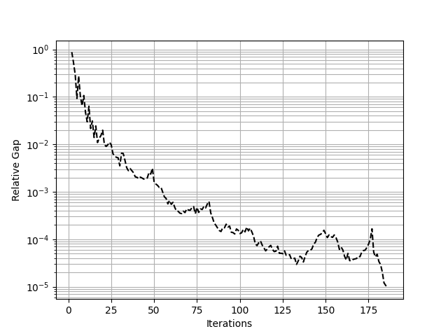
We can also plot convergence
import matplotlib.pyplot as plt

df = assig.report()
x = df.iteration.values
y = df.rgap.values

fig = plt.figure()
ax = fig.add_subplot(111)

plt.plot(x, y, "k--")
plt.yscale("log")
plt.grid(True, which="both")
plt.xlabel(r"Iterations")
plt.ylabel(r"Relative Gap")
plt.show()
Close the project
project.close()
Total running time of the script: ( 0 minutes 3.718 seconds)