Traffic Assignment

Similar to other complex algorthms that handle a large amount of data through complex computations, traffic assignment procedures can always be subject to at least one very reasonable question: Are the results right?

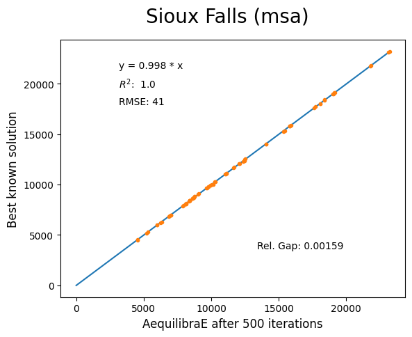
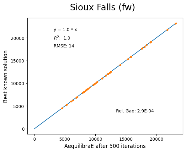
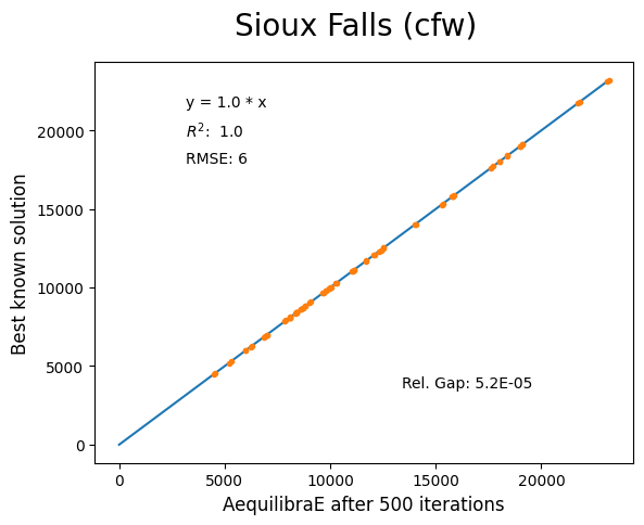
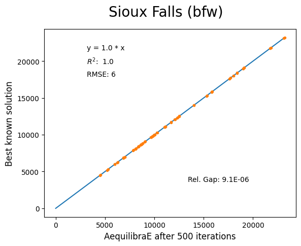
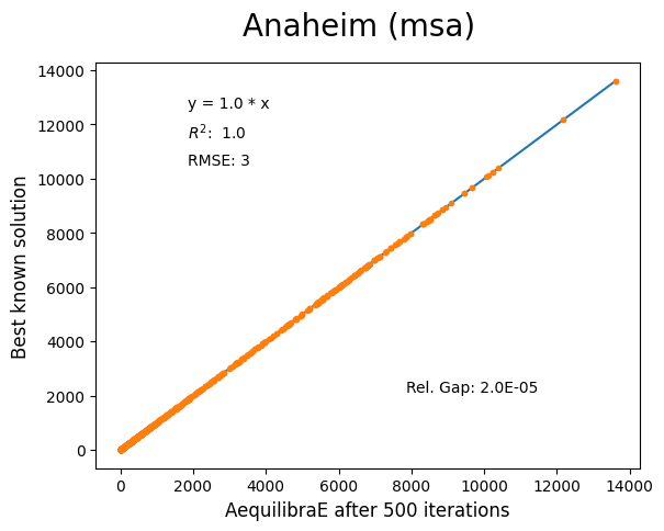
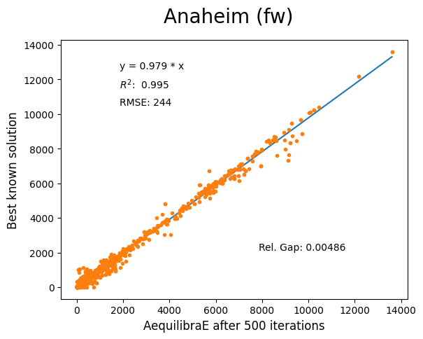
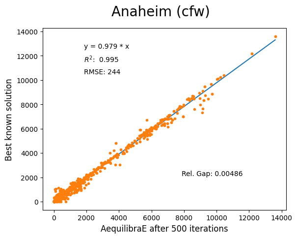
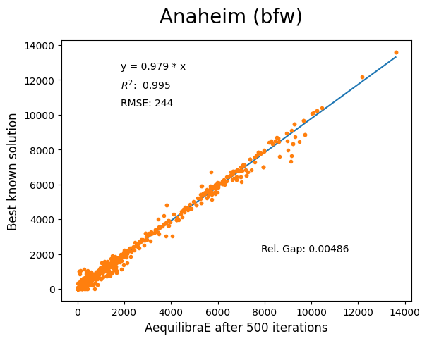
For this reason, we have used all equilibrium traffic assignment algorithms available in AequilibraE to solve standard instances used in academia for comparing algorithm results, some of which have are available with highly converged solutions (~1e-14). Instances can be downloaded here.

Sioux Falls

Network has:

• Links: 76

• Nodes: 24

• Zones: 24

Anaheim

Network has:

• Links: 914

• Nodes: 416

• Zones: 38

Winnipeg

Network has:

• Links: 914

• Nodes: 416

• Zones: 38

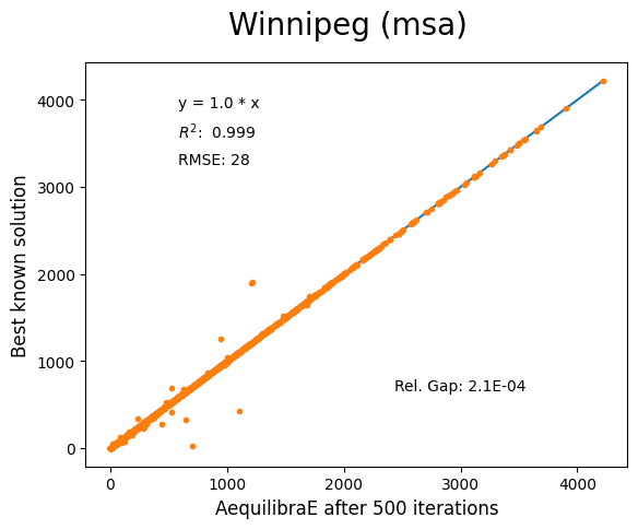
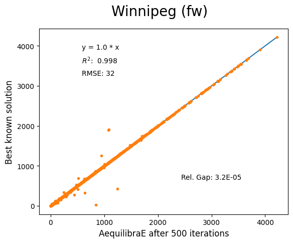
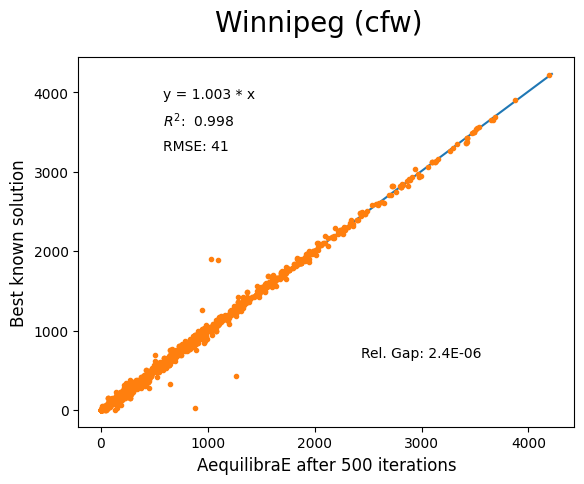
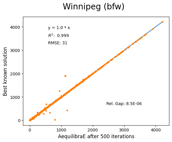
The results for Winnipeg do not seem extremely good when compared to a highly, but we believe posting its results would suggest deeper investigation by one of our users :-)

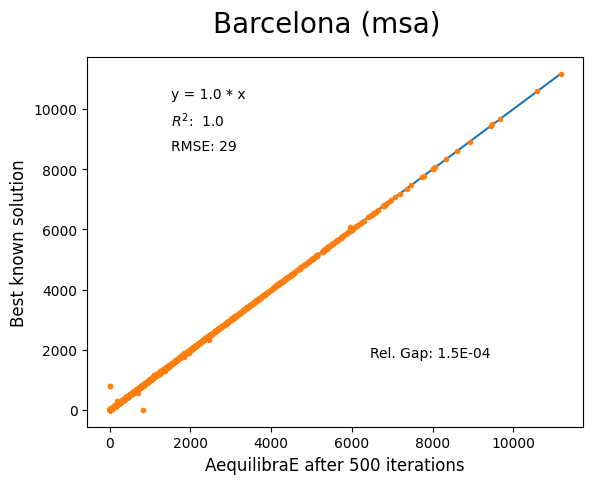
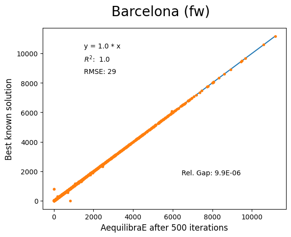
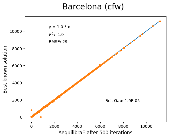
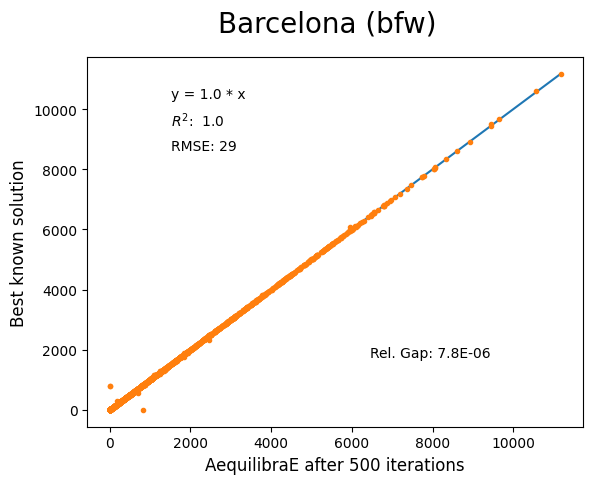
Barcelona

Network has:

• Links: 2,522

• Nodes: 1,020

• Zones: 110

Chicago Regional

Network has:

• Links: 39,018

• Nodes: 12,982

• Zones: 1,790

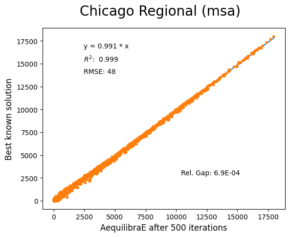
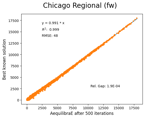
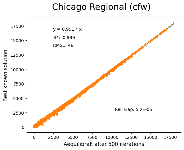
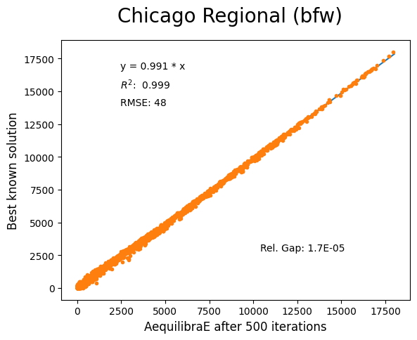
Convergence Study

Besides validating the final results from the algorithms, we have also compared how well they converge for the largest instance we have tested (Chicago Regional), as that instance has a comparable size to real-world models.

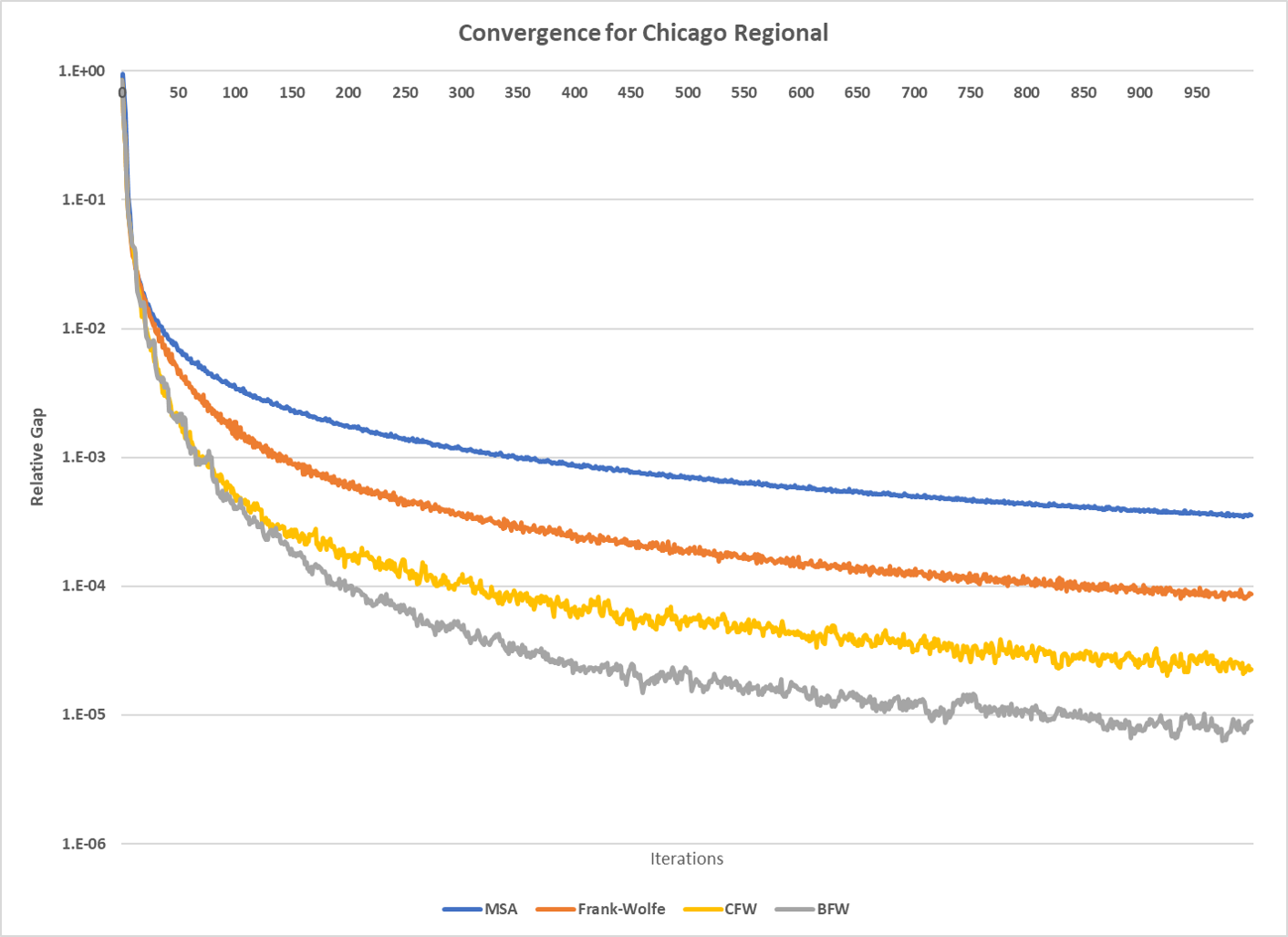
Not surprinsingly, one can see that Frank-Wolfe far outperforms the Method of Successive Averages for a number of iterations larger than 25, and is capable of reaching 1.0e-04 just after 800 iterations, while MSA is still at 3.5e-4 even after 1,000 iterations.

The actual show, however, is left for the Biconjugate Frank-Wolfe implementation, which delivers a relative gap of under 1.0e-04 in under 200 iterations, and a relative gap of under 1.0e-05 in just over 700 iterations.

This convergence capability, allied to its computational performance described below suggest that AequilibraE is ready to be used in large real-world applications.

Computational performance

Running on a IdeaPad laptop equipped with a 6 cores (12 threads) Intel Core i7-10750H CPU @ 2.60 GHz, and 32GB of RAM, AequilibraE performed 1,000 iterations of Frank-Wolfe assignment on the Chicago Network in just under 18 minutes, while Bi-conjugate Frank Wolfe takes just under 19 minutes, or a little more than 1s per All-or-Nothing iteration.

Compared with AequilibraE previous versions, we can notice a reasonable decrease in processing time.

Noteworthy items

Note

The biggest opportunity for performance in AequilibraE right now it to apply network contraction hierarchies to the building of the graph, but that is still a long-term goal

Want to run your own convergence study?

If you want to run the convergence study in your machine, with Chicago Regional instance or any other instance presented here, check out the code block below! Please make sure you have already imported TNTP files into your machine.

In the first part of the code, we’ll parse TNTP instances to a format AequilibraE can understand, and then we’ll perform the assignment.

# Imports
import os
import numpy as np
import pandas as pd
from aequilibrae.matrix import AequilibraeMatrix, AequilibraeData

from aequilibrae.paths import TrafficAssignment
from aequilibrae.paths.traffic_class import TrafficClass
import statsmodels.api as sm

from aequilibrae.paths import Graph
from copy import deepcopy

# Folders
data_folder = 'C:/your/path/to/TransportationNetworks/chicago-regional'
matfile = os.path.join(data_folder, 'ChicagoRegional_trips.tntp')

# Creating the matrix
f = open(matfile, 'r')
all_rows = f.read()
blocks = all_rows.split('Origin')[1:]
matrix = {}
for k in range(len(blocks)):
    orig = blocks[k].split('\n')
    dests = orig[1:]
    orig=int(orig[0])

    d = [eval('{'+a.replace(';',',').replace(' ','') +'}') for a in dests]
    destinations = {}
    for i in d:
        destinations = {**destinations, **i}
    matrix[orig] = destinations
zones = max(matrix.keys())
index = np.arange(zones) + 1
mat = np.zeros((zones, zones))
for i in range(zones):
    for j in range(zones):
        mat[i, j] = matrix[i+1].get(j+1,0)

# Let's save our matrix in AequilibraE Matrix format
aemfile = os.path.join(folder, "demand.aem")
aem = AequilibraeMatrix()
kwargs = {'file_name': aem_file,
        'zones': zones,
        'matrix_names': ['matrix'],
        "memory_only": False}  # in case you want to save the matrix in your machine

aem.create_empty(**kwargs)
aem.matrix['matrix'][:,:] = mtx[:,:]
aem.index[:] = index[:]

# Now let's parse the network
net = os.path.join(data_folder, 'ChicagoRegional_net.tntp')
net = pd.read_csv(net, skiprows=7, sep='\t')

network = net[['init_node', 'term_node', 'free_flow_time', 'capacity', "b", "power"]]
network.columns = ['a_node', 'b_node', 'free_flow_time', 'capacity', "b", "power"]
network = network.assign(direction=1)
network["link_id"] = network.index + 1

# If you want to create an AequilibraE matrix for computation, then it follows
g = Graph()
g.cost = net['free_flow_time'].values
g.capacity = net['capacity'].values
g.free_flow_time = net['free_flow_time'].values

g.network = network
g.network.loc[(g.network.power < 1), "power"] = 1
g.network.loc[(g.network.free_flow_time == 0), "free_flow_time"] = 0.01
g.network_ok = True
g.status = 'OK'
g.prepare_graph(index)
g.set_graph("free_flow_time")
g.set_skimming(["free_flow_time"])
g.set_blocked_centroid_flows(True)

# We run the traffic assignment
for algorithm in ["bfw", "fw", "cfw", "msa"]:

    mat = AequilibraeMatrix()
    mat.load(os.path.join(data_folder, "demand.aem"))
    mat.computational_view(["matrix"])

    assigclass = TrafficClass("car", g, mat)

    assig = TrafficAssignment()

    assig.set_classes([assigclass])
    assig.set_vdf("BPR")
    assig.set_vdf_parameters({"alpha": "b", "beta": "power"})
    assig.set_capacity_field("capacity")
    assig.set_time_field("free_flow_time")
    assig.max_iter = 1000
    assig.rgap_target = 1e-10
    assig.set_algorithm(algorithm)

    assig.execute()
    assigclass.results.save_to_disk(
        os.path.join(data_folder, f"convergence_study/results-1000.aed"))

    assig.report().to_csv(os.path.join(data_folder, f"{algorithm}_computational_results.csv"))

As we’ve exported the assignment’s results into CSV files, we can use Pandas to read the files, and plot a graph just like the one above.