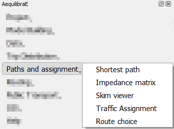
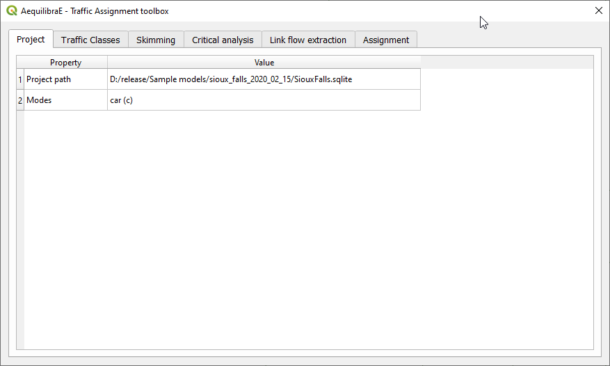
Paths and Assignment#

From version 0.6, AequilibraE plugin does not require the user to create the graph to perform path computation as in previous versions. In this version, as you set up your own configurations, the software already computes the graph for you.

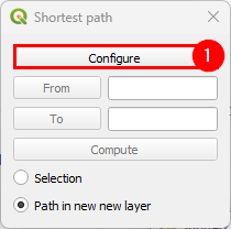
Shortest Path#

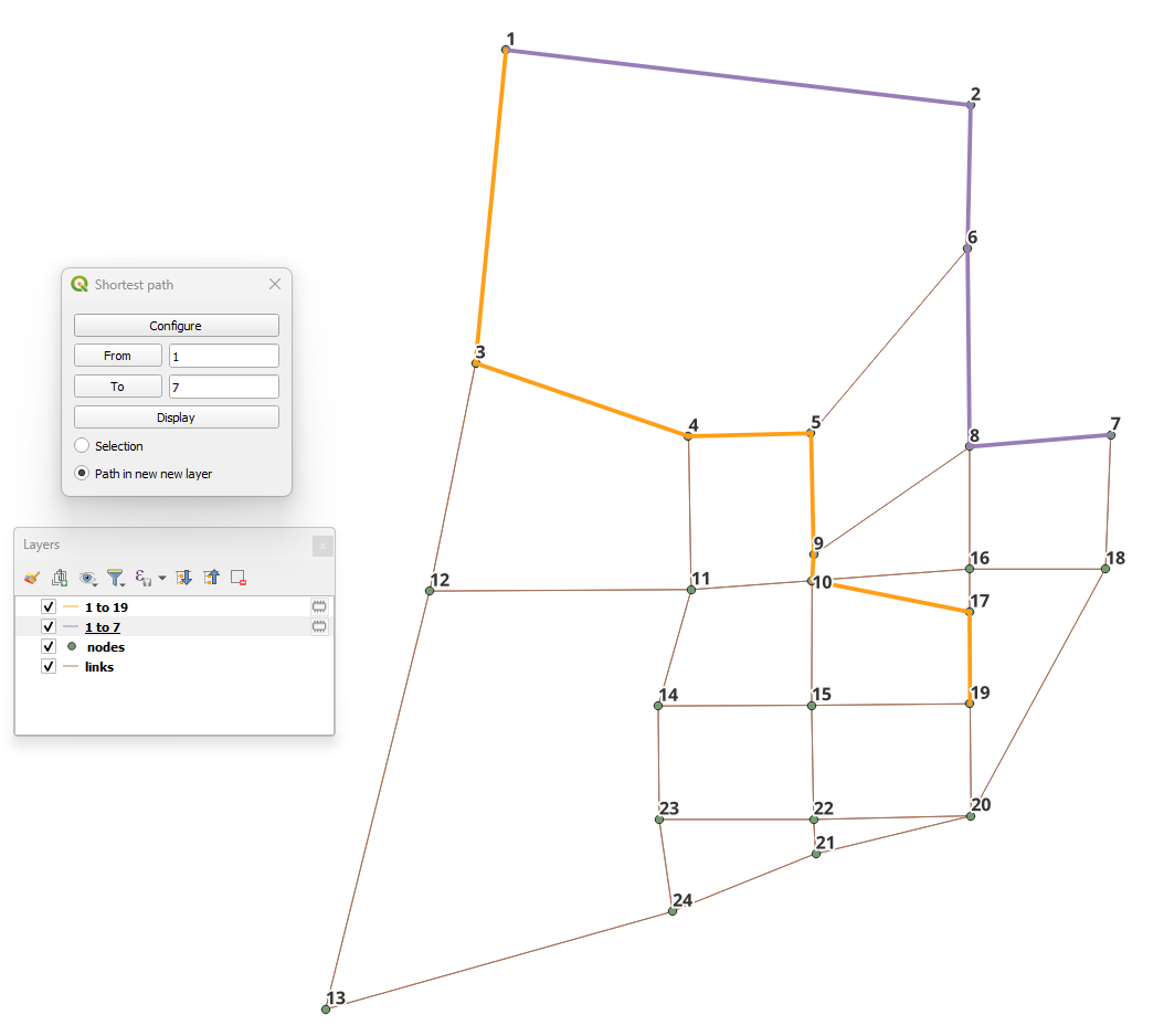
The first thing we can do with this project is to compute a few arbitrary paths to see if the network is connected and if paths make sense.

Before computing a path, we go to the configuration screen.

For the case of Sioux Falls, we need to configure the graph to accept paths going through centroids (all nodes are centroids), but that is generally not the case. For zones with a single connector per zone it is slightly faster to also deselect this option, but use this carefully.

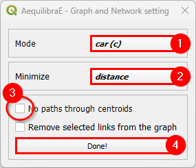
If we select that paths need to be in a separate layer, then every time you compute a path, a new layer with a copy of the links in that path will be created and formatted in a noticeable way. You can also select to have links selected in the layer, but only one path can be shown at time if you do so.

Impedance Matrix (aka Skimming Matrix)#

We can also skim the network to look into general connectivity of the network.

To perform skimming, we can select to compute a matrix from all nodes to all nodes, or from centroids to centroids, as well as to not allow flows through centroids.

The main controls, however, are the mode to skim, the field we should minimize when computing shortest paths and the fields we should skim when computing those paths.

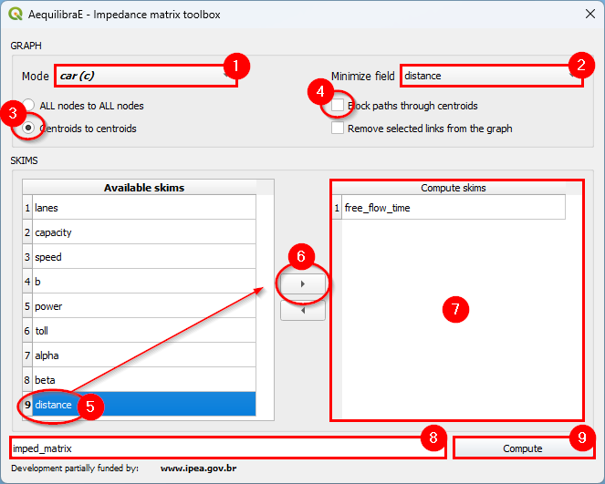
With the results computed (AEM or OMX), one can display them on the screen, loading the data using the non-project data tab in Data > Visualize data.

Skim viewer#

The skim viewer makes it easier to view skimming results. The skim viewer window looks like this:

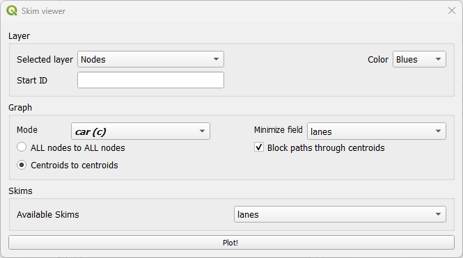
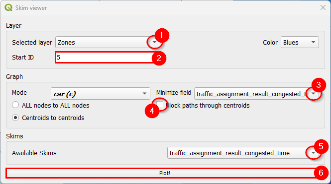
In the Layer group, you can select between the nodes or zones layers for data viewing. You can also select a color map range for plotting and the starting node/zone ID.

In the Graph group, you can set the graph configurations, such as the mode, the minimizing (cost) field, the choice to block or allow flows through the centroids, and whether to compute skims for all nodes or between centroids. Another useful feature of the skim viewer is that it allows users to use joined fields from the ‘links’ layer as minimizing or skimming fields.

Finally, in the Skim group, you select the desired skimming field for plotting.

When visualizing the skims, you’ll notice that a memory layer named ‘skim_viewer’ is created. It contains the node or zone ID for joining the nodes or zones layer and a data column that holds the data to be plotted. Whenever the selected node or zone changes, the values in the data column also change.

Skim view without joined layer#

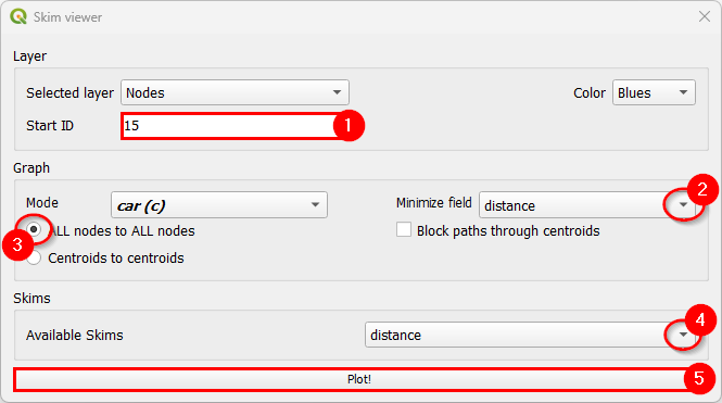
For demonstration purposes, we’ll use the Coquimbo model for this example. You can go directly to the skim viewer and set the configuration, as presented below:

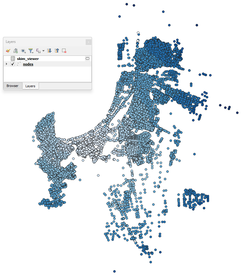
The output in the map canvas is:

If you select any other node with the skim viewer window open in the background, you will notice that the image displayed in the map canvas automatically changes.

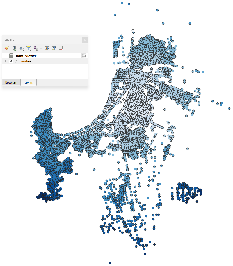
If you want to change either the minimizing field or skimming field (or both), you can modify your selection directly in the skim viewer window, and it will be automatically recomputed for display in the map canvas.

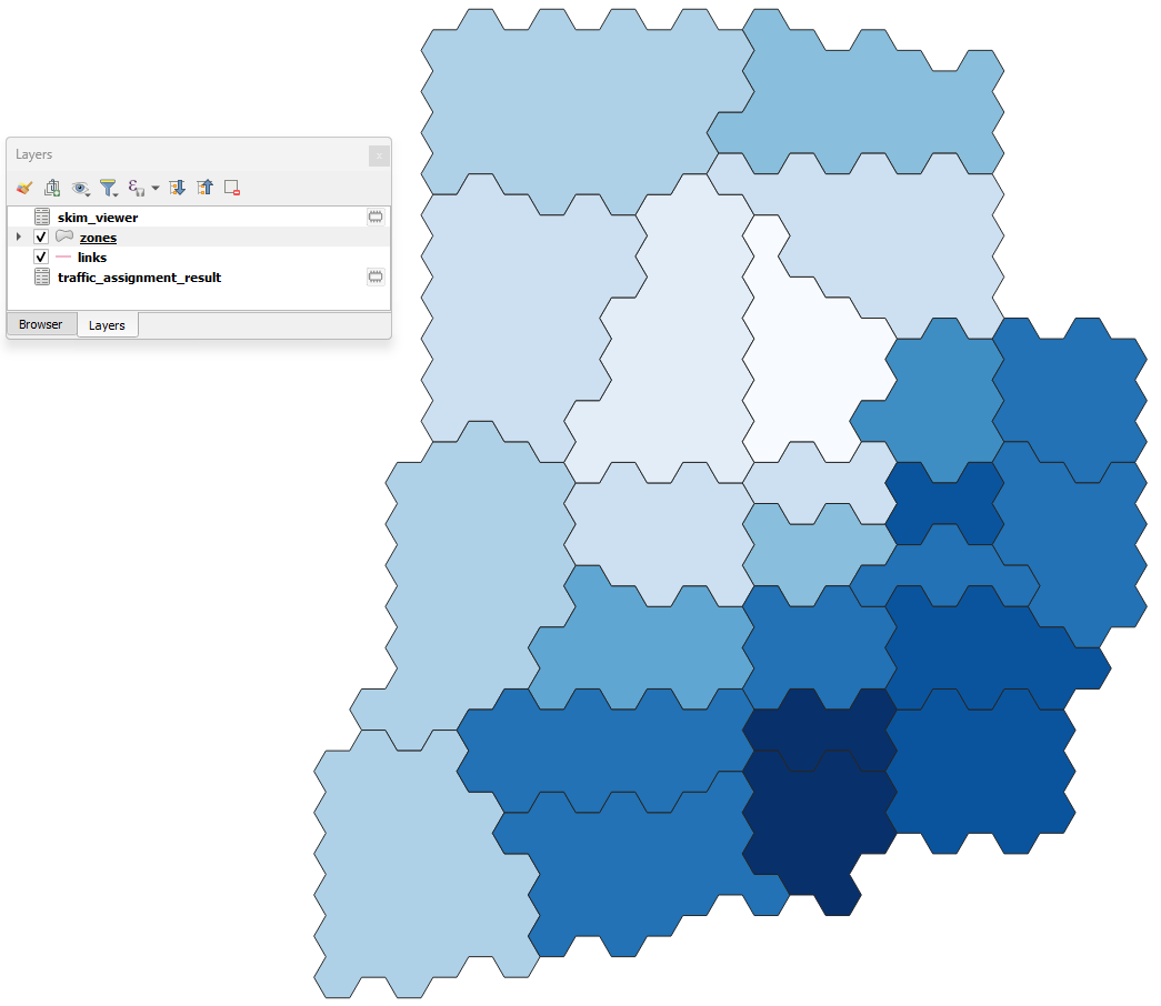
Skim viewer with joined layer#

For this example, we’ll use the Sioux Falls model. First, join the ‘links’ layer with the desired results table (see Visualize data for more information). Then, go to the skim viewer. When you see the window for the first time, you won’t notice anything different, but when you click on the minimize field and available skims, you’ll notice that the joined fields also appear here.

Let’s plot the zones for Sioux Falls, starting at zone ID 5, and using traffic_assignment_result_congested_time for both the costs and skimming fields. The initial configuration looks like this:

The output in the map canvas will be:

If your zone layer is active and you select another zone with the skim viewer window open in the background, you’ll notice that the image in the map canvas automatically changes.

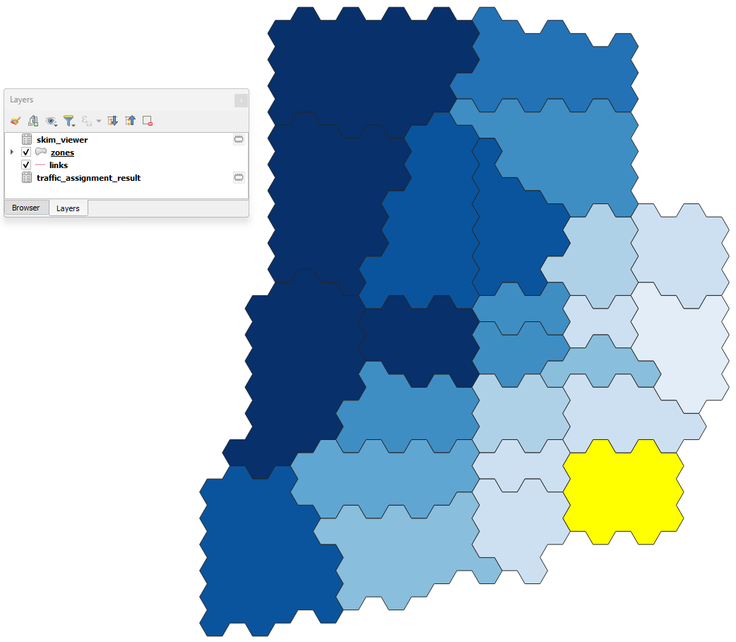
If you want to change either the minimizing field or skimming field (or both), you can modify your selection directly in the skim viewer window, and it will be automatically recomputed for display in the map canvas.

Traffic assignment#

Having verified that the network seems to be in order, one can proceed to perform traffic assignment, since we have a demand matrix.

The Traffic Assignment procedure tab looks like this!

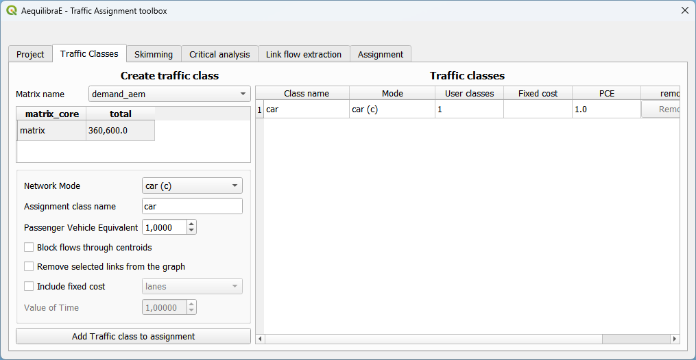
In the Traffic Classes tab you will create the traffic classes used in the project. First, select one of the available matrices (in *.AEM or *.OMX format), and the matrix core that will be used for computation. For the Sioux Falls example, we don’t want to block flow through centroids, but this is only necessary because regular nodes of the network are centroids. When you finish, just press the Add Traffic class to assignment button.

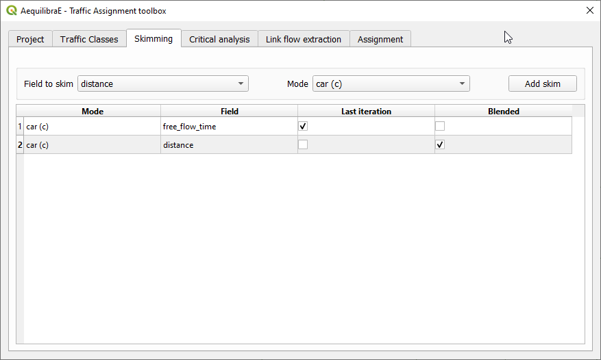
To select skims, we need to choose which fields/modes we will skim

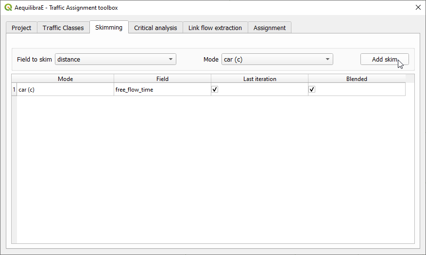
And if we want the skim for the last iteration (like we would for time) or if we want it averaged out for all iterations (properly averaged, that is).

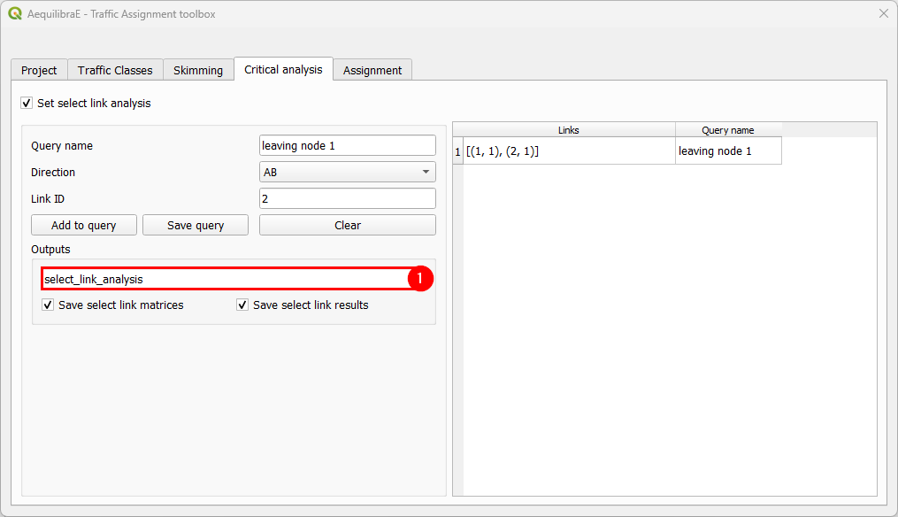
Next, we can choose to run a select link analysis. Its default configuration is not to select any links, so we have to toggle its “Set select link analysis” button.

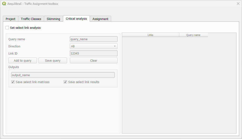
The creation of queries for analysis consists in: create a name for the query, select the travel direction, add the link ID, and click on Add to query, to temporarily save the data to the query.

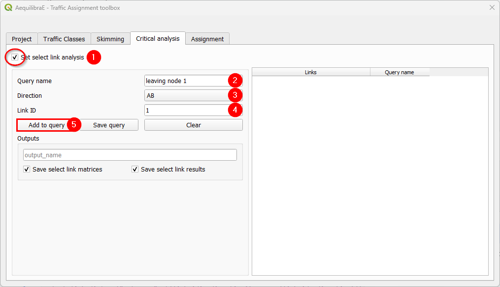
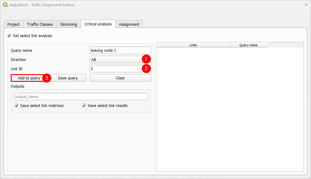
Adding more links to the previous query is straightforward. Select the direction and the link ID, and press Add to query once again.

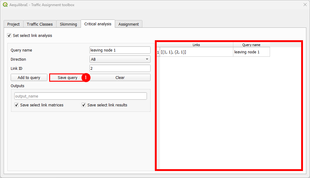
When we are done with the current query, we click on Save query, and notice that the query with the selected links is going to appear in the right-hand side table.

To finish the select link analysis step, we choose one name to save one or both of the matrix and results files.

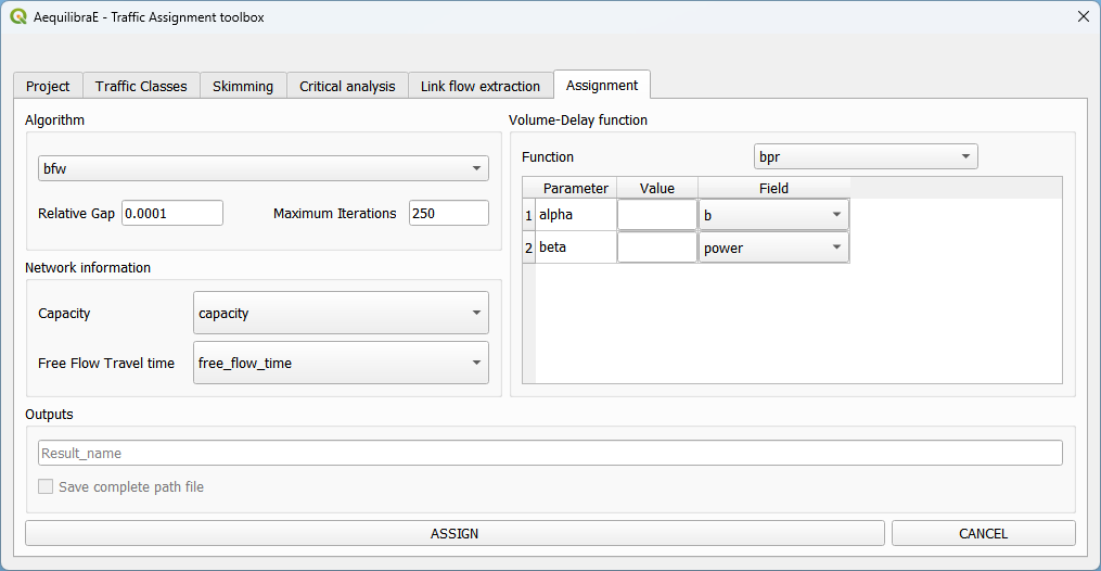
The final step is to setup the assignment itself.

Here we select the fields for:

link capacity
link free flow travel time
BPR’s alpha
BPR’s beta

We also confirm the Relative gap and maximum number of iterations we want, the assignment algorithm and the output folder. In this case, we again choose to not block flows through centroids for the reason discussed above.

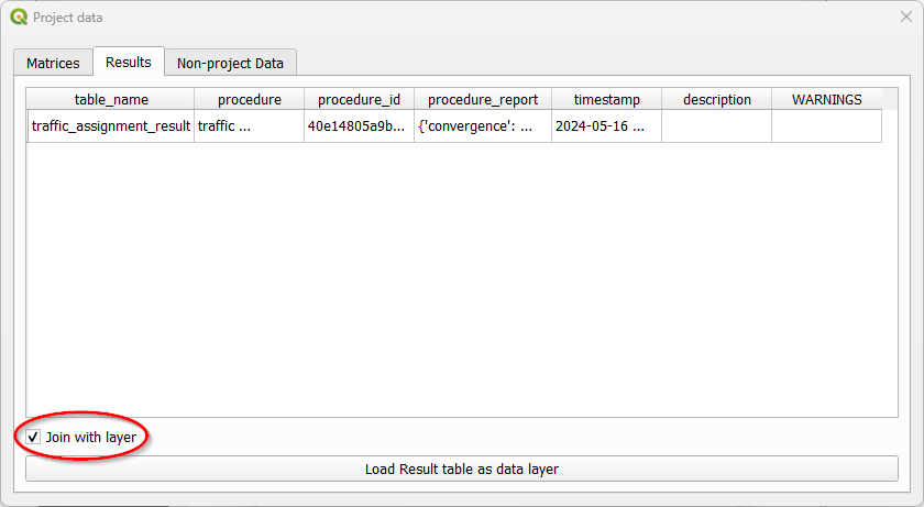
The result of the traffic assignment we just performed is stored in the results.sqlite database within the project folder. It can be easily accessed and loaded by clicking Data > Visualize data, and a project data window will open. Just click on the Results tab, select the desired result, let the Join with layer option checked, and click in the Load Result table as data layer button at the bottom. The result table layer will be automatically joined with the links layer.

Now we can revisit the instructions for Stacked Bandwidth

Route choice#

With the route choice sub-module, it is possible to create choice sets with three different algorithms as well as assign trips to the network using the traditional path-size logit. Using this module in QAequilibraE is trivial

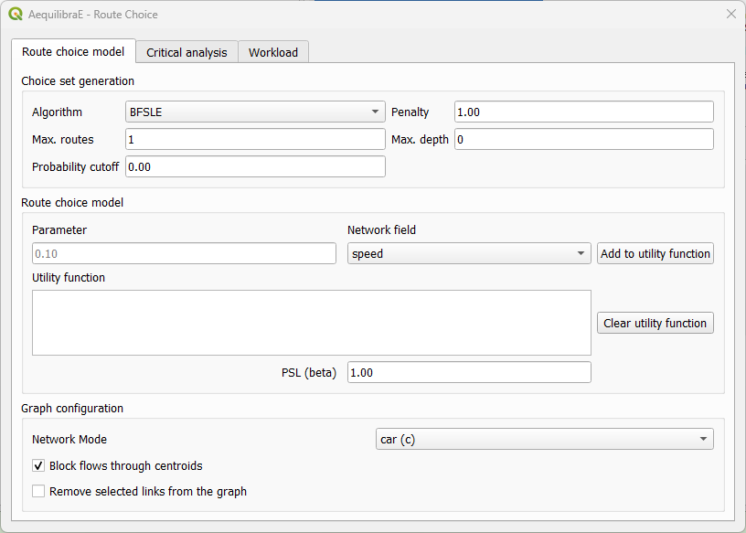
In the tab “Route choice model”, we add the model configuration. It consists of three different boxes. In the first box “Choice set generation”, we input parameters for the choice set construction. In the “Route choice model”, we add the parameters for the route choice model, such as the utility function and the path overlap parameter (PSL/beta) value. Finally, in “Graph configuration” we set up the graph used for computation.

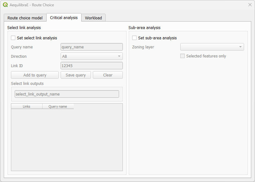
In the tab “Critical analysis”, we can select to run either a set of select link analysis or a sub-area analysis. These analyses cannot be run at the same time in QAequilibraE. If you choose to run a sub-area analysis, all OD pairs with demand are considered for computation. To select only a few pairs of interest, we encourage you to take a look at Route choice with sub-area analysis at AequilibraE’s Python documentation and run this task outside QGIS.

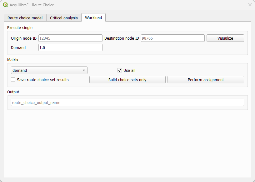
Lastly, the tab “Workload” allows users to choose between three tasks. The first box, “Execute single” consists of computing route choices between two different nodes and visualizing it, while the second box “Matrix” allows the selection of a travel demand matrix to be assigned using the route choice specified. This option also allows the user to save choice sets to disk while performing route choice.

We can run different workflows with the route choice sub-model. We’ll briefly present them.

Basic route choice#

In this example, we’ll perform route choice for the Coquimbo example model for a single OD pair. As this example model does not ship with a demand matrix, we can manually create an open layer and use its data to import the matrix to the project, as shown in Importing matrices to project.

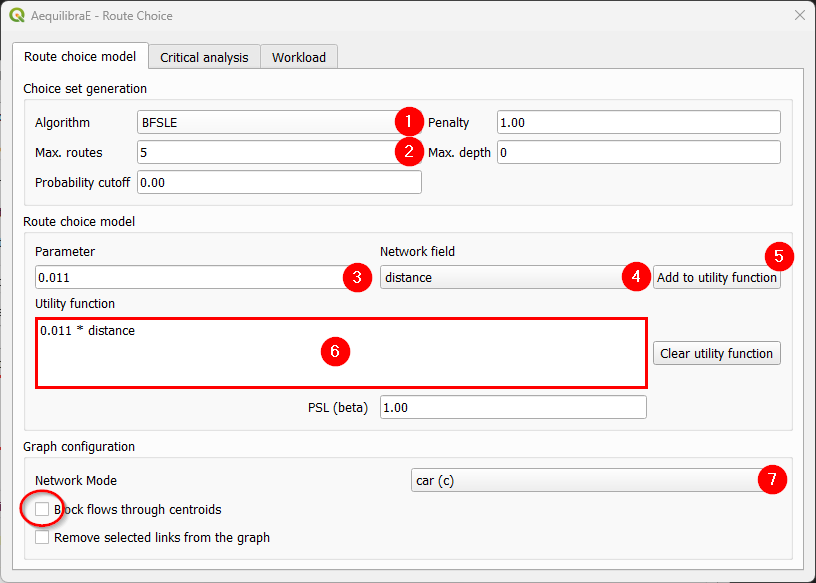
We start by setting the route choice parameters. In the “Choice set generation” box, we select the algorithm to be one of Link Penalization (LP), Breadth-First Link Search on Link Elimination (BFSLE), or BFSLE with LP, choose the values for probability cutoff and penalty, and choose a positive value for one of maximum number of routes (LP) or search depth (BFSLE and BFSLE + LP).

In the box “Route choice model” box, we configure our utility function. In this example, it is a function of distance, but could be any other numeric field, such as travel time or tolls. We then add the parameters to the utility function and it will appear in the utility function box. We can change the utility function by cleaning it and adding it one more time. To add more parameters to the utility function, just change the values and click in “Add to utility function” one more time.

Regarding “Graph configuration”, we’ll use the network for cars and allow flows through centroids.

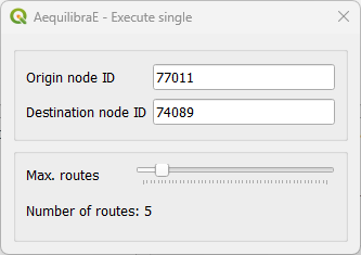
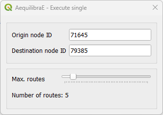
We can now move directly to the “Workload”, select origin and destination nodes and click on the visualize button.

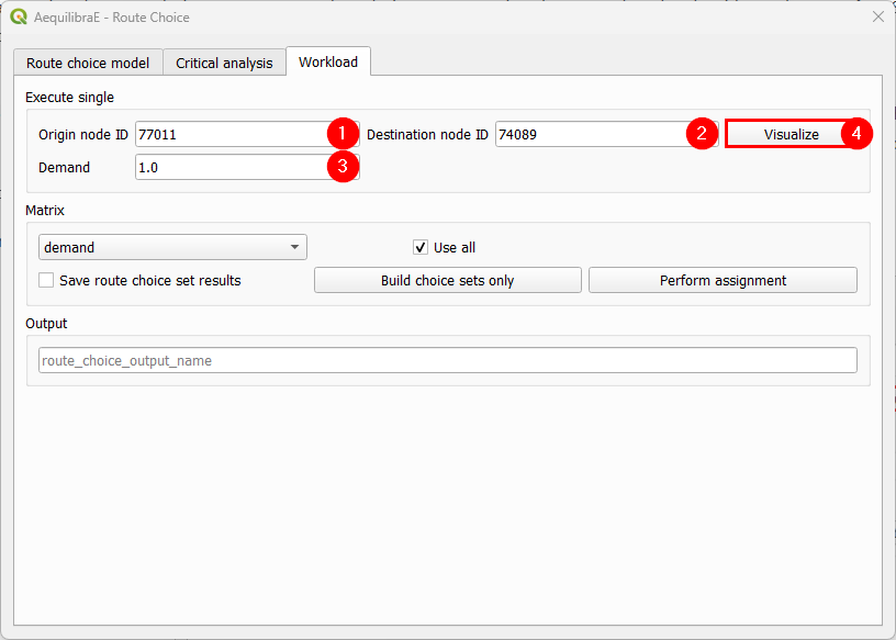
A new window named Execute Single will appear, loading the configuration we just used for the route choice set. If we are done with the choice set generation, we can close it, otherwise, we can generate the route choice set for another OD pair, also setting the desired number of routes.

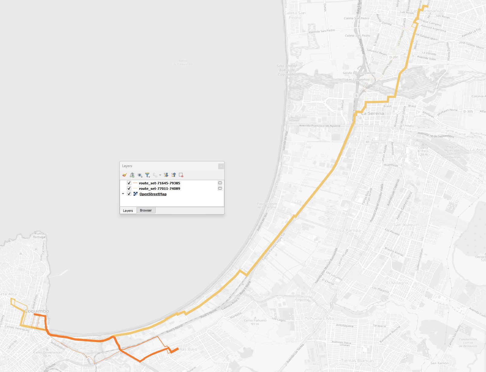
Basic route choice - execute single dialog - first OD pair

Basic route choice - execute single dialog - new OD pair

After a few seconds, the output visualization for the routes is shown in the map canvas and we can close the Execute Single window. The figure below presents the route choice sets, in which the line width corresponds to the probability of choosing each link.

Build choice sets#

Within this workflow, we can build and save the choice sets without performing assignment. We start by configuring the model parameters, then go to the “Workload” tab and select our demand matrix and its cores for computation.

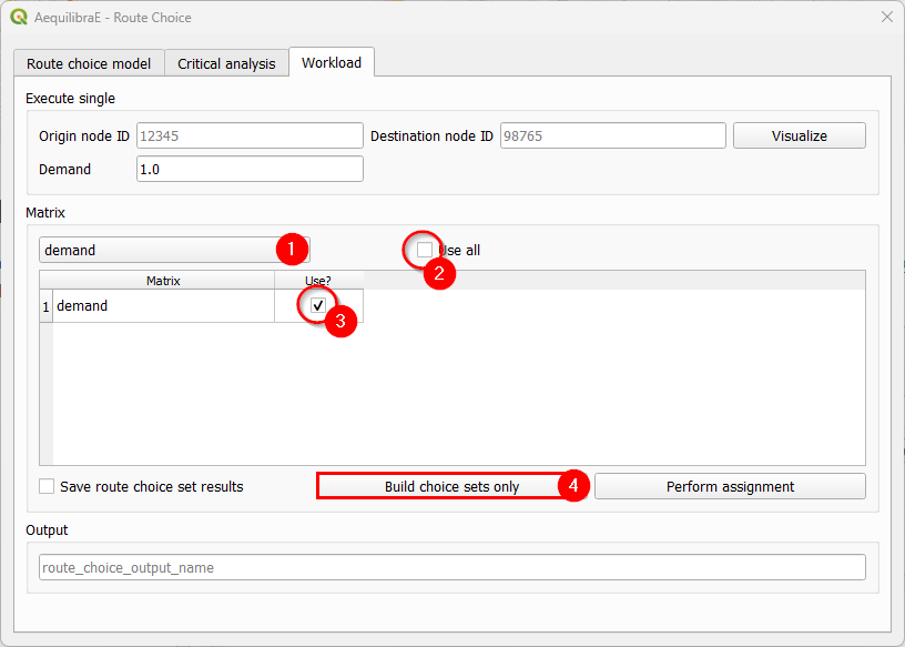
If you want to use all cores for computation, just let the “Use all” checkbox untoggled after choosing the matrix. Otherwise a table with the matrix cores and if they should be used is opened and we can select the cores we want.

Then all we need to do is hit the “Build choice sets only”. Once the task is finished, our route choice window will automatically close. If you go to the project folder, you will notice that a folder named ‘route choice’ containing folders with the choice sets for each centroid (index) in the matrix was created.

It should be noted that, although we are not performing assignment in this workflow, we use demand matrices to determine the OD pairs for which choice sets are needed, which are all of those with positive demand.

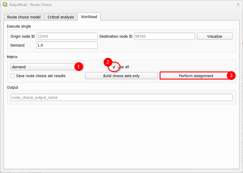
Perform assignment#

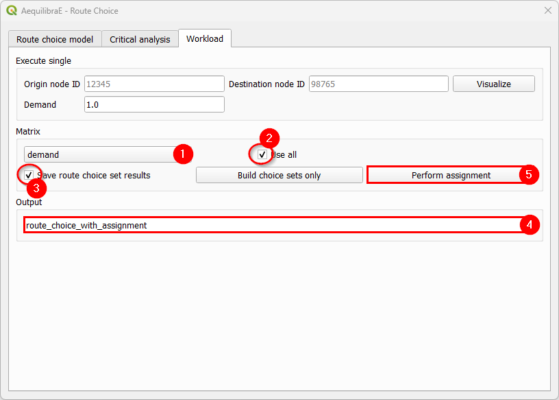
This workflow runs a route choice assignment and allows the user to save the choice set generated while performing such. The set up is quite similar to the one above: After setting the model parameters up, we go straight to the “Workload” tab and select the demand matrix and its cores for computation.

In this example, we choose to also save the choice sets generated, by toggling the “Save route choice set results” button. If we leave this button untoggled, only link flows are saved into the results database.

We also choose a name for saving the results in the database. Pick up a name that you can easily find later. Then, just hit the button “Perform assignment” and wait until the window is closed and the process is finished.

Select link analysis#

The left portion of the “Critical analysis” tab gives the user access to select link analysis. Its interface is quite similar to the one in Traffic Assignment, in which we can add and remove queries with selected links, and save both the matrix and the results in the databse.

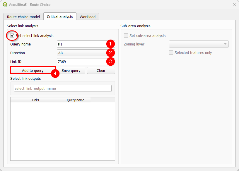
We start by toggling the “Set select link analysis” checkbox and enabling the following menus.

Let’s add our first query. Create a name, set the link direction, add the link ID, and click on “Add to query”.

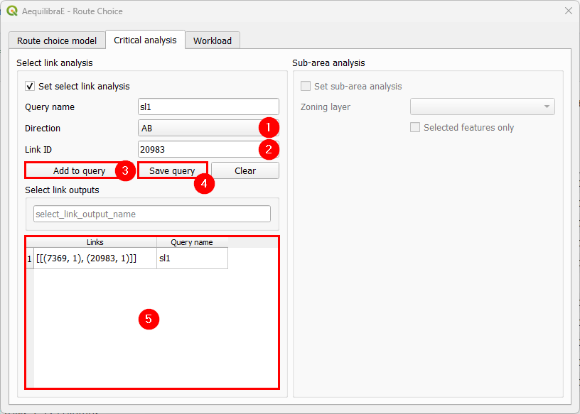
Let’s add another link to our SL1 query. Let’s set the link direction and link ID, add to the existing query with “Add to query”, and click on “Save query” (4). The SL1 query will immediately appear in the table at the bottom of the window (5).

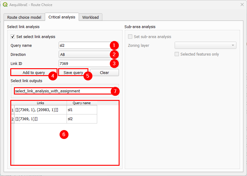
Just to make this example more interesting, let’s create an SL2 query. We repeat the process of creating a query name, setting the direction, selecting link ID, adding and saving the query. It will also appear at the bottom table (6). To remove any query from the query table, we can double-click the cell. Once this is our last query, we pick up a nice name to save our select link analysis results (7).

The last step consists in selecting the matrix and its cores for computation, and perform the assignment. It’s not necessary to add a name to the route choice output, once we did it in the previous step.

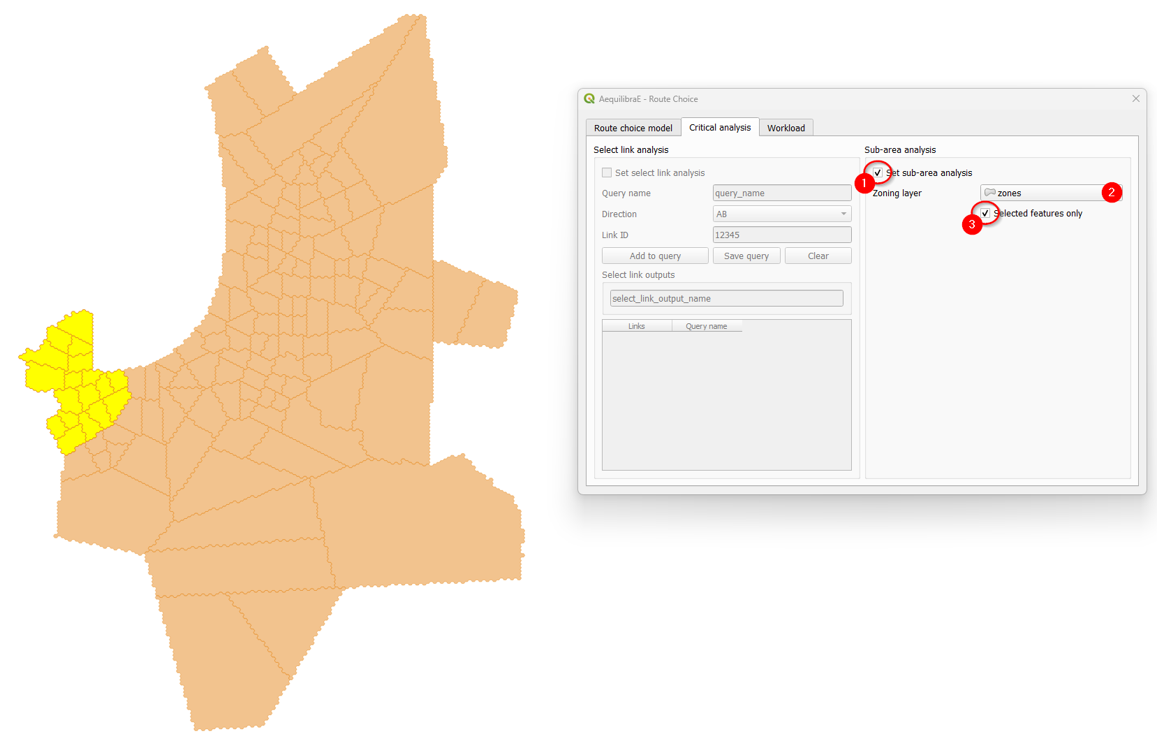
Sub-area analysis#

To perform a sub-area analysis, we start by toggling the “Set sub-area analysis” checkbox, which enables us to choose a polygon layer that defines the sub-area of interest. In this example, we select a couple zones in Coquimbo, and toggle the checkbox “Selected features only”. We could also use an external polygon layer with the desired region and use all the layer features rather than a part of it.

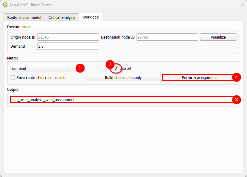
Finally, select all cores of our demand matrix for computation, don’t forget to add a name for the output file, and hit the “Perform assignment” button. When the process is finished, the window is closed. If you go to the project folder, you will notice that a folder named ‘route choice’ containing a .parquet file with the same output name you selected in (3) containing the sub-area demand matrix.

Tip

Try to reproduce AequilibraE’s Route Choice examples in QGIS!