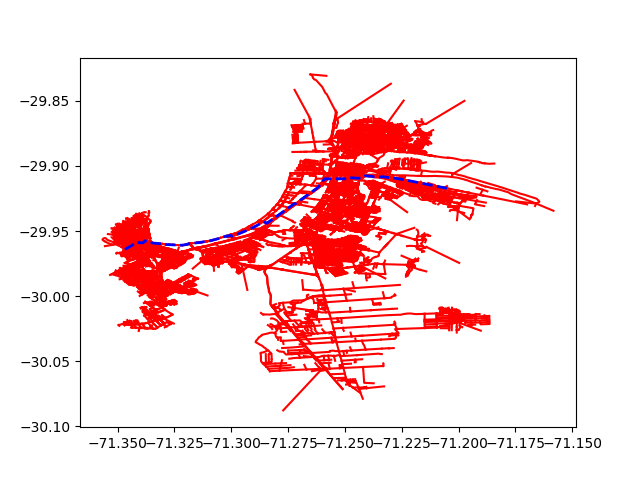
Path computation

In this example, we show how to perform path computation for Coquimbo, a city in La Serena Metropolitan Area in Chile.

# Imports
from uuid import uuid4
from tempfile import gettempdir
from os.path import join
from aequilibrae.utils.create_example import create_example

# We create the example project inside our temp folder
fldr = join(gettempdir(), uuid4().hex)

project = create_example(fldr, "coquimbo")

import logging
import sys

# We the project opens, we can tell the logger to direct all messages to the terminal as well
logger = project.logger
stdout_handler = logging.StreamHandler(sys.stdout)
formatter = logging.Formatter("%(asctime)s;%(levelname)s ; %(message)s")
stdout_handler.setFormatter(formatter)
logger.addHandler(stdout_handler)

Path Computation

from aequilibrae.paths import PathResults

We build all graphs

project.network.build_graphs()
# We get warnings that several fields in the project are filled with NaNs.
# This is true, but we won't use those fields.

/opt/hostedtoolcache/Python/3.9.18/x64/lib/python3.9/site-packages/aequilibrae/project/network/network.py:342: FutureWarning: Downcasting object dtype arrays on .fillna, .ffill, .bfill is deprecated and will change in a future version. Call result.infer_objects(copy=False) instead. To opt-in to the future behavior, set `pd.set_option('future.no_silent_downcasting', True)`
  df = pd.read_sql(sql, conn).fillna(value=np.nan)
2024-02-25 08:38:15,285;WARNING ; Field(s) speed, travel_time, capacity, osm_id, lanes has(ve) at least one NaN value. Check your computations
2024-02-25 08:38:15,371;WARNING ; Field(s) speed, travel_time, capacity, osm_id, lanes has(ve) at least one NaN value. Check your computations
2024-02-25 08:38:15,473;WARNING ; Field(s) speed, travel_time, capacity, osm_id, lanes has(ve) at least one NaN value. Check your computations
2024-02-25 08:38:15,573;WARNING ; Field(s) speed, travel_time, capacity, osm_id, lanes has(ve) at least one NaN value. Check your computations

We grab the graph for cars

graph = project.network.graphs["c"]

# we also see what graphs are available
# project.network.graphs.keys()

# let's say we want to minimize the distance
graph.set_graph("distance")

# And will skim time and distance while we are at it
graph.set_skimming(["travel_time", "distance"])

# And we will allow paths to be computed going through other centroids/centroid connectors
# required for the Sioux Falls network, as all nodes are centroids
# BE CAREFUL WITH THIS SETTING
graph.set_blocked_centroid_flows(False)

Let’s instantiate a path results object and prepare it to work with the graph

res = PathResults()
res.prepare(graph)

# compute a path from node 32343 to 22041, thats from near the airport to Fort Lambert, a popular location due to its views of the Coquimbo bay.
res.compute_path(32343, 22041)

# We can get the sequence of nodes we traverse
res.path_nodes

array([32343, 79778, 68225, 32487, 63937, 63192, 46510, 32380, 32373,
       55817, 55816, 11982, 46516, 75015, 79704, 79785, 78576, 68242,
       79144, 78635, 79784, 78748, 79082, 65861, 78343, 21311, 20312,
       21308, 78834, 79862, 79450, 63873, 79458, 78986, 78884, 79152,
       78645, 78549, 68503, 13380, 13383, 79199, 79745, 79457, 80001,
       78217, 78093, 80013, 25130, 80012, 40633, 11010, 11009, 40846,
       21827, 80056, 80055, 79481, 79486, 79485, 75142, 11448, 11446,
       11445, 67684, 60645, 11447, 11422, 11420, 11421, 13723, 10851,
       79462, 26681, 13718, 12079, 79460, 23707, 29778, 75451, 75445,
       45342, 39399, 13626, 13627, 45379, 21384, 63812, 40005, 12207,
       44243, 44241, 23405, 60002, 27114, 79431, 15148, 15146, 60000,
       75486, 55963, 55958, 59043, 59050, 59988, 39402, 59017, 59019,
       79398, 75520, 75516, 75512, 75509, 75505, 75511, 63544, 63543,
       75510, 75515, 75476, 63539, 30138, 11695, 61061, 30148, 44192,
       75556, 79364, 75534, 75552, 75548, 75321, 75532, 14802, 14823,
       71435, 65497, 64708, 64709, 64712, 64713, 40374, 40375, 77308,
       65518, 75566, 68526, 75573, 41306, 41308, 75619, 75617, 14899,
       14875, 38674, 75595, 65067, 65068, 79508, 29452, 44797, 29447,
       10065, 44798, 30552, 44783, 44808, 75612, 73617, 79653, 79651,
       73620, 73923, 79820, 14864, 69009, 22040, 22041])

# We can get the link sequence we traverse
res.path

array([34709, 34710, 34711, 34712, 34713, 34714, 34715, 34716, 34717,
       34718, 34719, 34720, 34721, 34722,  3321,  3322,  3323,  3324,
        3325,  3326,  3327,  3328,  3329,  3330,  3331,  3332,  2970,
        2971,  2969, 19995,  1434,  1435,  1436, 19326, 19327, 19328,
       19329, 19330, 33674, 33675, 33676, 33677, 26525, 20765, 20746,
       20747, 20748, 20749, 20750, 20751, 20752,   496,   497,   498,
         499,   500,   501, 10380, 15408,   553,   552,   633,   634,
         635,   630,   631,   632,   623,   624,   625,   626,   471,
        5363, 34169, 34170, 34171, 34785,  6466,  6465, 29938, 29939,
       29940, 29941,  1446,  1447,  1448,  1449,  1450,   939,   940,
         941,  9840,  9841, 26314, 26313, 26312, 26311, 26310, 26309,
       26308, 26307, 26306, 26305, 26304, 26303, 26302, 26301, 26300,
       34079, 34147, 29962, 26422, 26421, 26420,   765,   764,   763,
         762,   761,   760,   736, 10973, 10974, 10975,   725, 10972,
         727,   728, 26424,   733,   734, 29899, 20970, 20969, 20968,
       20967, 20966, 20965, 20964, 20963, 20962,  9584,  9583, 20981,
       21398, 20982, 20983, 20984, 20985, 10030, 10031, 10032, 10033,
       10034, 10035, 10036,    64,    65, 21260, 21261, 21262, 21263,
       21264, 21265, 21266,    33, 11145, 11146,    71,    72, 34529,
       34530, 34531, 28691, 28692, 28693,  3574])

# We can get the mileposts for our sequence of nodes
res.milepost

# Additionally we could also provide `early_exit=True` or `a_star=True` to `compute_path` to adjust its path finding behaviour.
# Providing `early_exit=True` will allow the path finding to quit once it's discovered the destination, this means it will
# perform better for ODs that are topographically close. However, exiting early may cause subsequent calls to `update_trace`
# to recompute the tree in cases where it usually wouldn't. `a_star=True` has precedence of `early_exit=True`.
res.compute_path(32343, 22041, early_exit=True)

# If you'd prefer to find a potentially non-optimal path to the destination faster provide `a_star=True` to use A* with a
# heuristic. With this method `update_trace` will always recompute the path.
res.compute_path(32343, 22041, a_star=True)



# By default a equirectangular heuristic is used. We can view the available heuristics via
res.get_heuristics()

# If you'd like the more accurate, but slower, but more accurate haversine heuristic you can set it using
res.set_heuristic("haversine")

# or
res.compute_path(32343, 22041, a_star=True, heuristic="haversine")

# If we want to compute the path for a different destination and the same origin, we can just do this
# It is way faster when you have large networks
# Here we'll adjust our path to the University of La Serena. Our previous early exit and A* settings will persist with calls
# to `update_trace`. If you'd like to adjust them for subsequent path re-computations set the `res.early_exit` and `res.a_star` attributes.
res.a_star = False
res.update_trace(73131)

res.path_nodes

array([32343, 79778, 68225, 32487, 63937, 63192, 46510, 32380, 32373,
       55817, 55816, 11982, 46516, 75015, 79704, 79785, 78576, 68242,
       79144, 78635, 79784, 78748, 79082, 65861, 78343, 21311, 20312,
       21308, 78834, 79862, 79450, 63873, 79458, 78986, 78884, 79152,
       78645, 78549, 68503, 13380, 13383, 79199, 79745, 79457, 80001,
       78217, 78093, 80013, 25130, 80012, 40633, 11010, 11009, 40846,
       21827, 80056, 80055, 79481, 79486, 79485, 75142, 11448, 11446,
       11445, 67684, 60645, 11447, 11422, 11420, 11421, 13723, 10851,
       79462, 26681, 13718, 12079, 79460, 23707, 29778, 75451, 75445,
       45342, 39399, 13626, 13627, 45379, 21384, 63812, 40005, 12207,
       44243, 44241, 23405, 60002, 27114, 79431, 15148, 15146, 60000,
       75486, 55963, 55958, 59043, 59050, 59988, 39402, 59017, 59019,
       79398, 75520, 75516, 75512, 75509, 75505, 75511, 63544, 63543,
       75510, 75515, 75476, 63539, 30138, 11695, 61061, 30148, 44192,
       75556, 79364, 75534, 75552, 75548, 75321, 75532, 14802, 14823,
       71435, 65497, 64708, 64709, 64712, 64713, 40374, 40375, 77308,
       65518, 75566, 68526, 79517, 51754, 77189, 65059, 10093, 65058,
       30491, 66966, 66863, 30492, 77190, 77191, 79366, 77417, 79368,
       77406, 77421, 77425, 77393, 77398, 53993, 77394, 70959, 77395,
       27752, 65293, 73131])

If you want to show the path in Python We do NOT recommend this, though…. It is very slow for real networks

import matplotlib.pyplot as plt
from shapely.ops import linemerge

links = project.network.links

# We plot the entire network
curr = project.conn.cursor()
curr.execute("Select link_id from links;")

for lid in curr.fetchall():
    geo = links.get(lid[0]).geometry
    plt.plot(*geo.xy, color="red")

path_geometry = linemerge(links.get(lid).geometry for lid in res.path)
plt.plot(*path_geometry.xy, color="blue", linestyle="dashed", linewidth=2)
plt.show()

project.close()