Trip Distribution

In this example, we calibrate a Synthetic Gravity Model that same model plus IPF (Fratar/Furness).

# Imports
from uuid import uuid4
from tempfile import gettempdir
from os.path import join
from aequilibrae.utils.create_example import create_example
import pandas as pd
import numpy as np

We create the example project inside our temp folder

fldr = join(gettempdir(), uuid4().hex)

project = create_example(fldr)

# We get the demand matrix directly from the project record
# so let's inspect what we have in the project
proj_matrices = project.matrices
print(proj_matrices.list())

         name      file_name  ...                           description status
0  demand_omx     demand.omx  ...  Original data imported to OMX format
1   demand_mc  demand_mc.omx  ...                                  None
2       skims      skims.omx  ...                          Example skim
3  demand_aem     demand.aem  ...  Original data imported to AEM format

[4 rows x 8 columns]

# We get the demand matrix
demand = proj_matrices.get_matrix("demand_omx")
demand.computational_view(["matrix"])

# And the impedance
impedance = proj_matrices.get_matrix("skims")
impedance.computational_view(["time_final"])

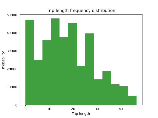
Let’s have a function to plot the Trip Length Frequency Distribution

from math import log10, floor
import matplotlib.pyplot as plt


def plot_tlfd(demand, skim, name):
    plt.clf()
    b = floor(log10(skim.shape[0]) * 10)
    n, bins, patches = plt.hist(
        np.nan_to_num(skim.flatten(), 0),
        bins=b,
        weights=np.nan_to_num(demand.flatten()),
        density=False,
        facecolor="g",
        alpha=0.75,
    )

    plt.xlabel("Trip length")
    plt.ylabel("Probability")
    plt.title("Trip-length frequency distribution")
    plt.savefig(name, format="png")
    return plt

from aequilibrae.distribution import GravityCalibration

for function in ["power", "expo"]:
    gc = GravityCalibration(matrix=demand, impedance=impedance, function=function, nan_as_zero=True)
    gc.calibrate()
    model = gc.model
    # We save the model
    model.save(join(fldr, f"{function}_model.mod"))

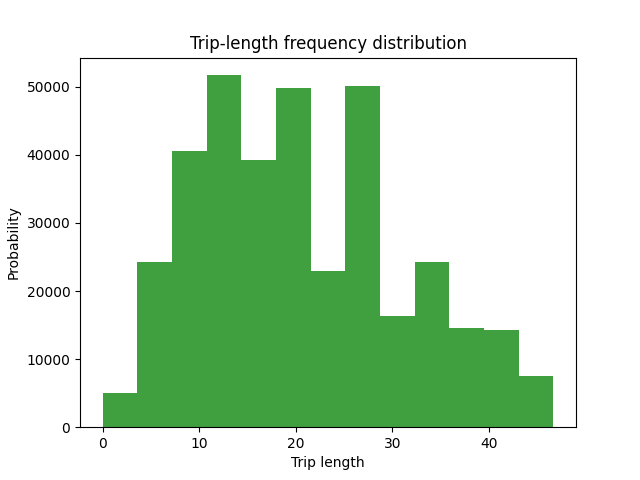
    # We can save an image for the resulting model
    _ = plot_tlfd(gc.result_matrix.matrix_view, impedance.matrix_view, join(fldr, f"{function}_tfld.png"))

    # We can save the result of applying the model as well
    # We can also save the calibration report
    with open(join(fldr, f"{function}_convergence.log"), "w") as otp:
        for r in gc.report:
            otp.write(r + "\n")

/opt/hostedtoolcache/Python/3.9.18/x64/lib/python3.9/site-packages/aequilibrae/distribution/gravity_application.py:318: RuntimeWarning: divide by zero encountered in power
  self.output.matrix_view[i, :] = (np.power(self.impedance.matrix_view[i, :], -self.model.alpha) * p * a)[
/opt/hostedtoolcache/Python/3.9.18/x64/lib/python3.9/site-packages/aequilibrae/distribution/gravity_application.py:332: RuntimeWarning: invalid value encountered in multiply
  self.output.matrix_view[:, :] = self.output.matrix_view[:, :] * non_inf

We save a trip length frequency distribution for the demand itself

plt = plot_tlfd(demand.matrix_view, impedance.matrix_view, join(fldr, "demand_tfld.png"))
plt.show()

Forecast

We create a set of ‘future’ vectors by applying some models and apply the model for both deterrence functions

from aequilibrae.distribution import Ipf, GravityApplication, SyntheticGravityModel
from aequilibrae.matrix import AequilibraeData
import numpy as np

zonal_data = pd.read_sql("Select zone_id, population, employment from zones order by zone_id", project.conn)
# We compute the vectors from our matrix

args = {
    "file_path": join(fldr, "synthetic_future_vector.aed"),
    "entries": demand.zones,
    "field_names": ["origins", "destinations"],
    "data_types": [np.float64, np.float64],
    "memory_mode": True,
}

vectors = AequilibraeData()
vectors.create_empty(**args)

vectors.index[:] = zonal_data.zone_id[:]

# We apply a trivial regression-based model and balance the vectors
vectors.origins[:] = zonal_data.population[:] * 2.32
vectors.destinations[:] = zonal_data.employment[:] * 1.87
vectors.destinations *= vectors.origins.sum() / vectors.destinations.sum()

# We simply apply the models to the same impedance matrix now
for function in ["power", "expo"]:
    model = SyntheticGravityModel()
    model.load(join(fldr, f"{function}_model.mod"))

    outmatrix = join(proj_matrices.fldr, f"demand_{function}_model.aem")
    args = {
        "impedance": impedance,
        "rows": vectors,
        "row_field": "origins",
        "model": model,
        "columns": vectors,
        "column_field": "destinations",
        "nan_as_zero": True,
    }

    gravity = GravityApplication(**args)
    gravity.apply()

    # We get the output matrix and save it to OMX too,
    gravity.save_to_project(name=f"demand_{function}_model_omx", file_name=f"demand_{function}_model.omx")

# We update the matrices table/records and verify that the new matrices are indeed there
proj_matrices.update_database()
print(proj_matrices.list())

                     name  ... status
0              demand_omx  ...
1               demand_mc  ...
2                   skims  ...
3              demand_aem  ...
4  demand_power_model_omx  ...
5   demand_expo_model_omx  ...

[6 rows x 8 columns]

We now run IPF for the future vectors

args = {
    "matrix": demand,
    "rows": vectors,
    "columns": vectors,
    "column_field": "destinations",
    "row_field": "origins",
    "nan_as_zero": True,
}

ipf = Ipf(**args)
ipf.fit()

ipf.save_to_project(name="demand_ipf", file_name="demand_ipf.aem")
ipf.save_to_project(name="demand_ipf_omx", file_name="demand_ipf.omx")

<aequilibrae.project.data.matrix_record.MatrixRecord object at 0x7ff1bdedc5e0>

print(proj_matrices.list())

                     name  ... status
0              demand_omx  ...
1               demand_mc  ...
2                   skims  ...
3              demand_aem  ...
4  demand_power_model_omx  ...
5   demand_expo_model_omx  ...
6              demand_ipf  ...
7          demand_ipf_omx  ...

[8 rows x 8 columns]

project.close()