The Transit assignment graph#

This page is a description of a graph structure for a transit network, used for static, link-based, frequency-based assignment. Our focus is the classic algorithm “Optimal strategies” by Spiess & Florian [1].

Let’s start by giving a few definitions:

transit definition from Wikipedia:

system of transport for passengers by group travel systems available for use by the general public unlike private transport, typically managed on a schedule, operated on established routes, and that charge a posted fee for each trip.

transit network: a set of transit lines and stops, where passengers can board, alight or change vehicles.
assignment: distribution of the passengers (demand) on the network (supply), knowing that transit users attempt to minimize total travel time, time or distance walking, time waiting, number of transfers, fares, etc…
static assignment : assignment without time evolution. Dynamic properties of the flows, such as congestion, are not well described, unlike with dynamic assignment models.
frequency-based (or headway-based) as opposed to schedule-based : schedules are averaged in order to get line frequencies. In the schedule-based approach, distinct vehicle trips are represented by distinct links. We can see the associated network as a time-expanded network, where the third dimension would be time.
link-based: the assignment algorithm is not evaluating paths, or any aggregated information besides attributes stored by nodes and links. In the present case, each link has an associated cost (travel time) c [s] and frequency f [1/s].

We are going at first to describe the input transit network, which is mostly composed of stops, lines and zones.

Elements of a transit network#

Transit stops and stations#

Transit stops are points where passenger can board, alight or change vehicles. Also, they can be part of larger stations:

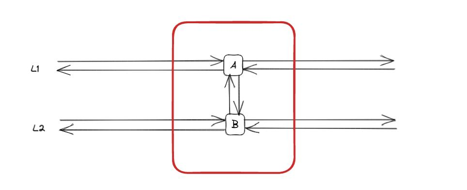
In the illustration above, two distinct stops, A and B, are highlighted, both affiliated with the same station (depicted in red).

Transit lines#

A transit line is a set of services that may use different routes, decomposed into segments.

Transit routes#

A routes is described by a sequence of stop nodes. We assume here the routes to be directed. For example, we can take a simple case with 3 stops:

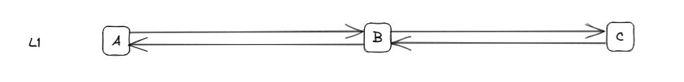
In this case, the L1 line is made of two distinct routes: - ABC - CBA.

Various configurations are possible, such as:

a partial route at a given moment of the day: AB,
a route with an additional stop : ABDC
a route that does not stop at a given stop: AC

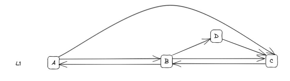
Lines can be decomposed into multiple sub-lines, each representing distinct routes. For the given example, we may have several sub-lines under the same commercial line (L1):

line id	commercial name	stop sequence	headway (s)
L1_a1	L1	ABC	600
L1_a2	L1	ABDC	3600
L1_a3	L1	AB	3600
L1_a4	L1	AC	3600
L1_b1	L1	CBA	600

Headway, associated with each sub-line, corresponds to the mean time range between consecutive vehicles—the inverse of the line frequency used as a link attribute in the assignment algorithm.

Line segments#

A line segment represents a portion of a transit line between two consecutive stops. Using the example line L1_a1, we derive two distinct line segments:

line id	segment index	origin stop	destination stop	travel_time (s)
L1_a1	1	A	B	300
L1_a1	2	B	C	600

Note that a travel time is included for each line segment, serving as another link attribute used by the assignment algorithm.

Transit assignment zones and connectors#

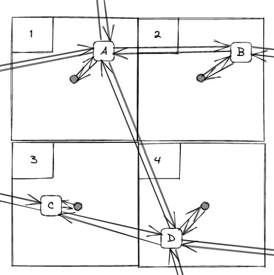
To effectively assign passengers on the network, expressing demand between regions is crucial. This is achieved by first decomposing the network area into a partition of transit assignment zones, as illustrated below with 4 non-overlapping zones:

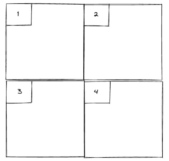
The demand is then expressed as a number of trips from each zone to every other zone, forming a 4 by 4 Origin/Destination (OD) matrix in this case.

Additionally, each zone centroid is connected to specific network nodes to facilitate the connection between supply and demand. These connection points are referred to as connectors.

With these components, we now have all the elements required to describe the assignment graph.

The Assignment graph#

Link and node types#

The transit network is used to generate a graph with specific nodes and links used to model the transit process. Various link types and node categories play crucial roles in this representation.

Link types:

on-board
boarding
alighting
dwell
transfer
connector
walking

Nodes types:

stop
boarding
alighting
od
walking

To illustrate, consider the anatomy of a simple stop:

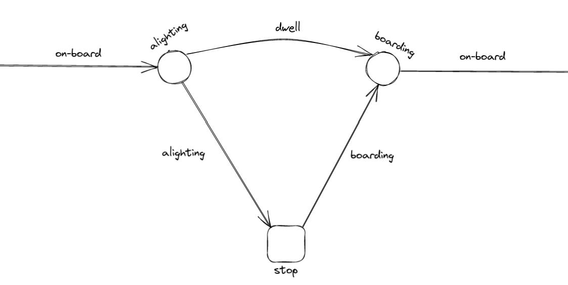
Waiting links encompass boarding and transfer links. Each line segment is associated with a boarding, an on-board and an alighting link.

Transfer links enable to compute the passenger flow count between line couples at the same stop:

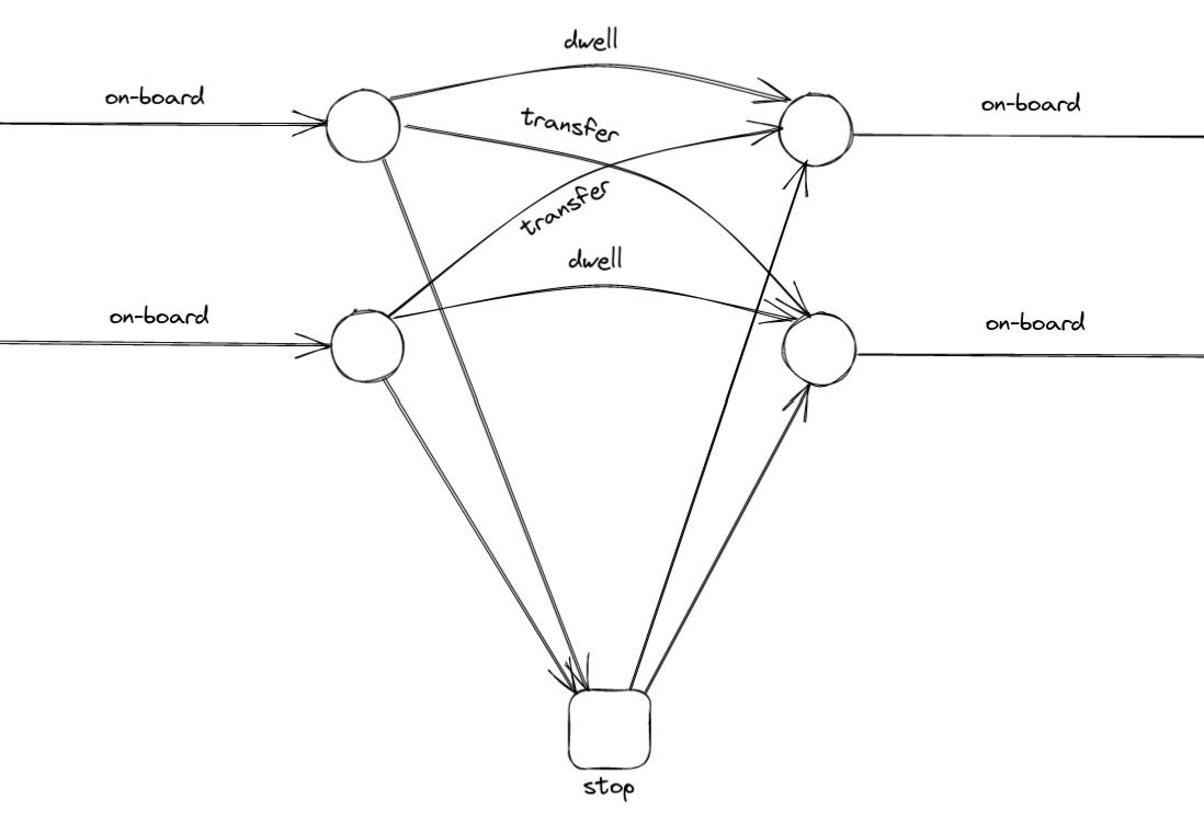
These links can be extended between all lines of a station if an increase in the number of links is viable.

walking links connect stop nodes within a station, while connector links connect the zone centroids (od nodes) to stop nodes:

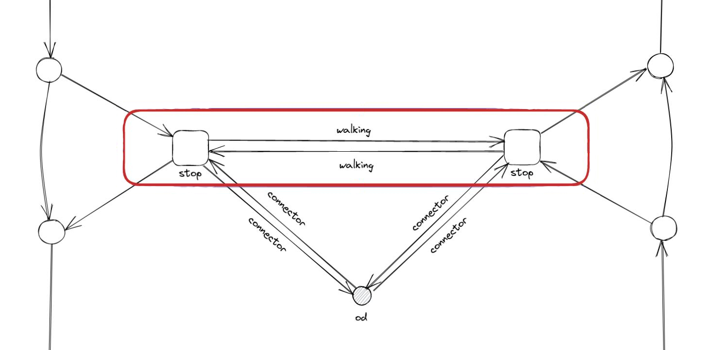
Connectors that connect od to stop nodes allow passengers to access the network, while connectors in the opposite direction allow them to egress. Walking nodes/links may also be used to connect stops from distant stations.

Link attributes#

The table below summarizes link characteristics and attributes based on link types:

link type	from node type	to node type	cost	frequency
on-board	boarding	alighting	trav. time	\(\infty\)
boarding	stop	boarding	const.	line freq.
alighting	alighting	stop	const.	\(\infty\)
dwell	alighting	boarding	const.	\(\infty\)
transfer	alighting	boarding	const. + trav. time	dest. line freq.
connector	od or stop	od or stop	trav. time	\(\infty\)
walking	stop or walking	stop or walking	trav. time	\(\infty\)

The travel time is specific to each line segment or walking time. For example, there can be 10 minutes connection between stops in a large transit station. Constant boarding and alighting times are applied uniformly across the network, and dwell links have constant cost equal to the sum of the alighting and boarding constants.

Additional attributes can be introduced for specific link types, such as:

line_id: for on-board, boarding, alighting and dwell links.
line_seg_idx: the line segment index for boarding, on-board and alighting links.
stop_id: for alighting, dwell and boarding links. This can also apply to transfer links for inner stop transfers.
o_line_id: origin line id for transfer links
d_line_id: destination line id for transfer links

In the next section, we will explore a small classic transit network example featuring four stops and four lines.

A Small example : Spiess and Florian#

This illustrative example is taken from Spiess and Florian [1]:

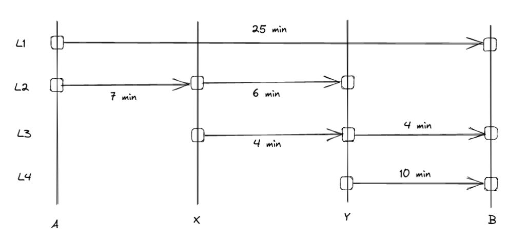
Travel time are indicated on the figure. We have the following four distinct line characteristics:

line id	route	headway (min)	frequency (1/s)
L1	AB	12	0.001388889
L2	AXY	12	0.001388889
L3	XYB	30	0.000555556
L4	YB	6	0.002777778

Passengers aim to travel from A to B, prompting the division of the network area into two distinct zones: TAZ 1 and TAZ 2. The assignment graph associated with this network encompasses 26 links:

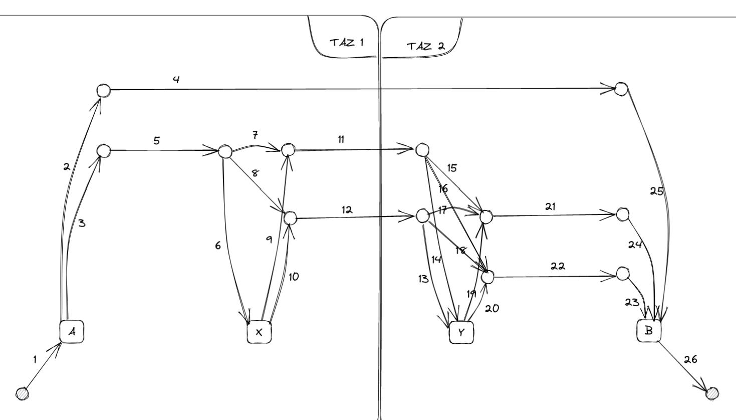
Here is a table listing all links :

link id	link type	line id	cost	frequency
1	connector		0	\(\infty\)
2	boarding	L1	0	0.001388889
3	boarding	L2	0	0.001388889
4	on-board	L1	1500	\(\infty\)
5	on-board	L2	420	\(\infty\)
6	alighting	L2	0	\(\infty\)
7	dwell	L2	0	\(\infty\)
8	transfer		0	0.000555556
9	boarding	L2	0	0.001388889
10	boarding	L3	0	0.000555556
11	on-board	L2	360	\(\infty\)
12	on-board	L3	240	\(\infty\)
13	alighting	L3	0	\(\infty\)
14	alighting	L2	0	\(\infty\)
15	transfer	L3	0	0.000555556
16	transfer		0	0.002777778
17	dwell	L3	0	\(\infty\)
18	transfer		0	0.002777778
19	boarding	L3	0	0.000555556
20	boarding	L4	0	0.002777778
21	on-board	L3	240	\(\infty\)
22	on-board	L4	600	\(\infty\)
23	alighting	L4	0	\(\infty\)
24	alighting	L3	0	\(\infty\)
25	alighting	L1	0	\(\infty\)
26	connector		0	\(\infty\)

Transit graph specificities in AequilibraE#

The graph creation process in AequilibraE incorporates several edge types to capture the nuances of transit networks. Notable distinctions include:

Connectors :

access connectors directed from od nodes to the network
egress connectors directed from the network to the od nodes

Transfer edges :

inner transfer: Connect lines within the same stop
outer transfer: Connect lines between distinct stops within the same station

Origin and Destination Nodes :

origin nodes: represent the starting point of passenger trips
destination nodes: represent the end point of passenger trips

Users can customize these features using boolean parameters:

with_walking_edges: create walking edges between the stops of a station
with_inner_stop_transfers: create transfer edges between lines of a stop
with_outer_stop_transfers: create transfer edges between lines of different stops of a station
blocking_centroid_flow: duplicate OD nodes into unconnected origin and destination nodes in order to block centroid flows. Flows starts from an origin node and ends at a destination node. It is not possible to use an egress connector followed by an access connector in the middle of a trip.

Note that during the assignment, if passengers have the choice between a transfer edge or a walking edge for a line change, they will always be assigned to the transfer edge.

This leads to these possible edge types:

on-board
boarding
alighting
dwell
access_connector
egress_connector
inner_transfer
outer_transfer
walking

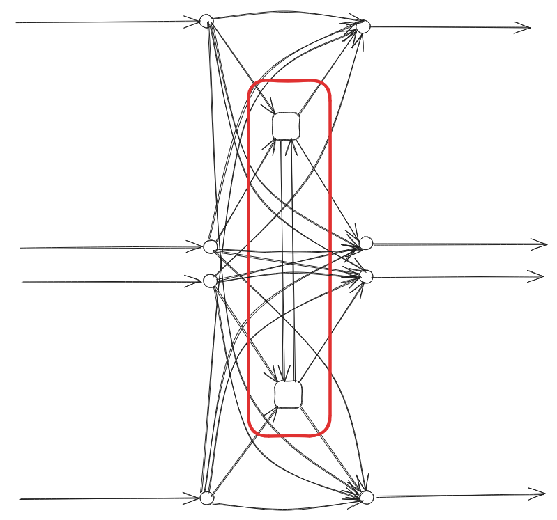
Here is a simple example of a station with two stops, with two lines each:

walking edges only:

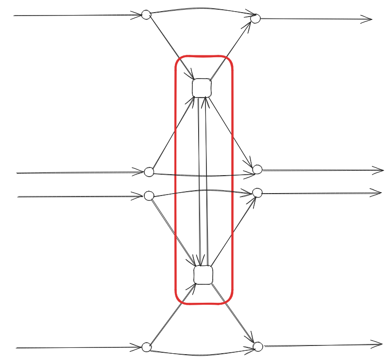
inner transfer edges, but no outer transfer ones:

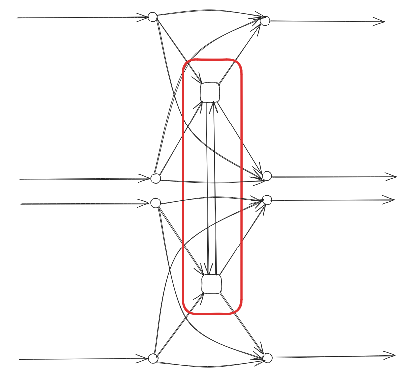
inner transfer edges, but no outer transfer edge

both inner and outer transfer edges:

As an illustrative example, if we build the graph for the city of Lyon France (GTFS files from 2022) on a given day, we get 20196 vertices and 91107 edges, with with_walking_edges=True, with_inner_stop_transfers=True, with_outer_stop_transfers=True and blocking_centroid_flow=False. Here is the distribution of edge types:

Edge type	Count
outer_transfer	27287
inner_transfer	10721
walking	9140
on-board	7590
boarding	7590
alighting	7590
dwell	7231
access_connector	6979
egress_connector	6979

and vertex types:

Vertex type	Count
alighting	7590
boarding	7590
stop	4499
od	517

References#

[1] Heinz Spiess, Michael Florian, Optimal strategies: A new assignment model for transit networks, Transportation Research Part B: Methodological, Volume 23, Issue 2, 1989, Pages 83-102, ISSN 0191-2615, https://doi.org/10.1016/0191-2615(89)90034-9.