Route choice

With the route choice sub-module, it is possible to create choice sets with three different algorithms as well as assign trips to the network using the traditional path-size logit. Using this module in QAequilibraE is trivial.

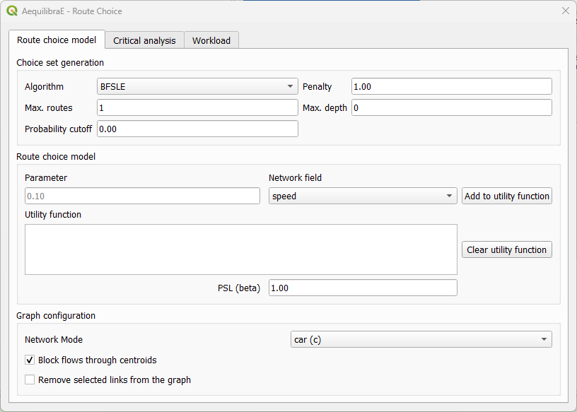
In the tab “Route choice model”, we add the model configuration. It consists of three different boxes. In the first box “Choice set generation”, we input parameters for the choice set construction. In the “Route choice model”, we add the parameters for the route choice model, such as the utility function and the path overlap parameter (PSL/beta) value. Finally, in “Graph configuration” we set up the graph used for computation.

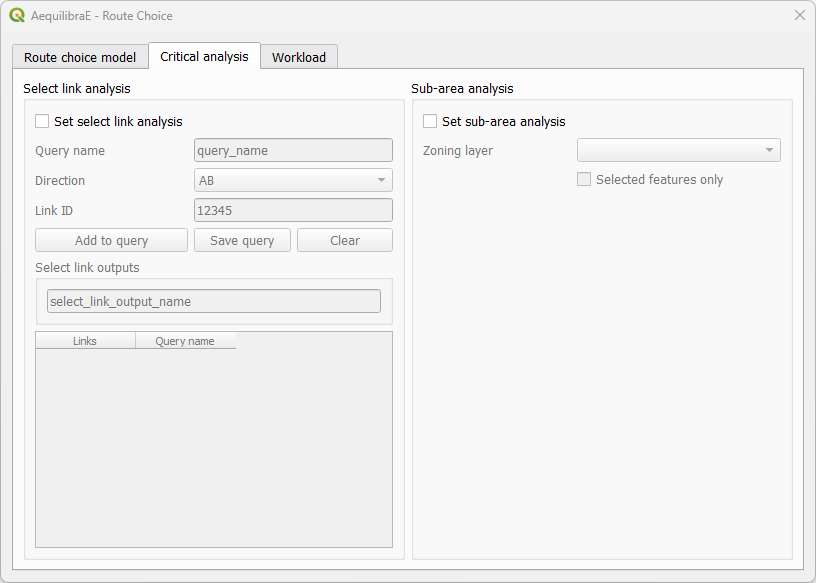
In the tab “Critical analysis”, we can select to run either a set of select link analysis or a sub-area analysis. These analyses cannot be run at the same time in QAequilibraE. If you choose to run a sub-area analysis, all OD pairs with demand are considered for computation. To select only a few pairs of interest, we encourage you to take a look at Route choice with sub-area analysis at AequilibraE’s Python documentation and run this task outside QGIS.

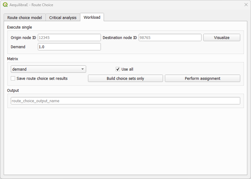
Lastly, the tab “Workload” allows users to choose between three tasks. The first box, “Execute single” consists of computing route choices between two different nodes and visualizing it, while the second box “Matrix” allows the selection of a travel demand matrix to be assigned using the route choice specified. This option also allows the user to save choice sets to disk while performing route choice.

Basic workflow

Basic route choice

In this example, we’ll perform route choice for the Coquimbo example model for a single OD pair. As this example model does not ship with a demand matrix, we can manually create an open layer and use its data to import the matrix to the project, as shown in Importing matrices.

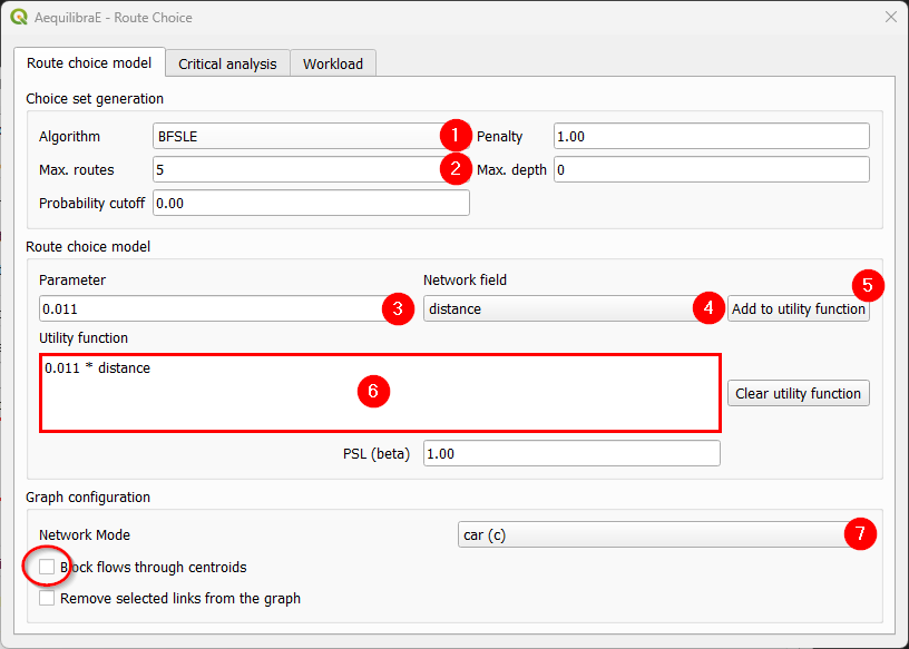
We start by setting the route choice parameters. In the “Choice set generation” box, we select the algorithm to be one of Link Penalization (LP), Breadth-First Link Search on Link Elimination (BFSLE), or BFSLE with LP, choose the values for probability cutoff and penalty, and choose a positive value for one of maximum number of routes (LP) or search depth (BFSLE and BFSLE + LP).

In the box “Route choice model” box, we configure our utility function. In this example, it is a function of distance, but could be any other numeric field, such as travel time or tolls. We then add the parameters to the utility function and it will appear in the utility function box. We can change the utility function by cleaning it and adding it one more time. To add more parameters to the utility function, just change the values and click in “Add to utility function” one more time.

Regarding “Graph configuration”, we’ll use the network for cars and allow flows through centroids.

We can now move directly to the “Workload”, select origin and destination nodes and click on the visualize button.

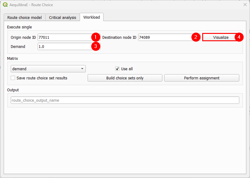
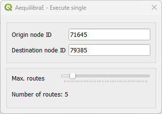
A new window named Execute Single will appear, loading the configuration we just used for the route choice set. If we are done with the choice set generation, we can close it, otherwise, we can generate the route choice set for another OD pair, also setting the desired number of routes.

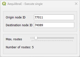
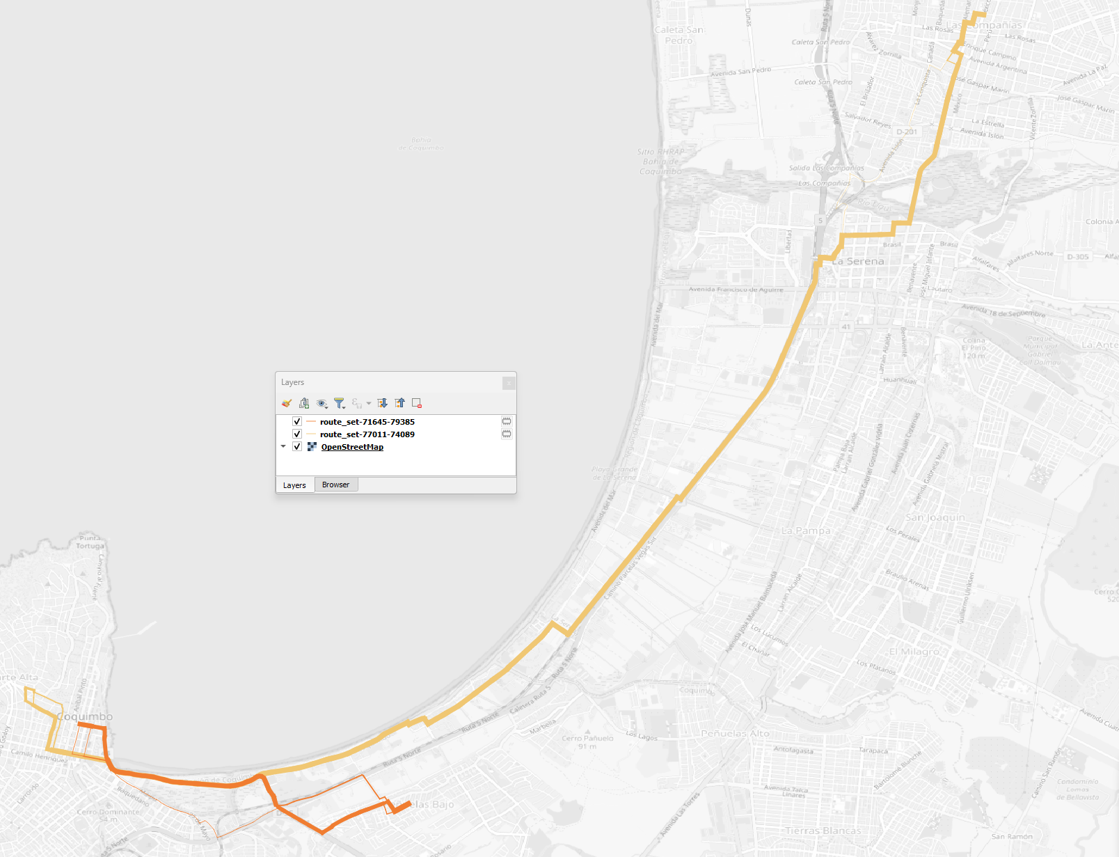
After a few seconds, the output visualization for the routes is shown in the map canvas and we can close the Execute Single window. The figure below presents the route choice sets, in which the line width corresponds to the probability of choosing each link.

Build choice sets

Within this workflow, we can build and save the choice sets without performing assignment. We start by configuring the model parameters, then go to the “Workload” tab and select our demand matrix and its cores for computation.

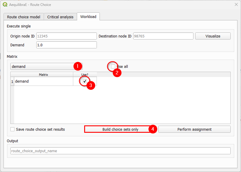
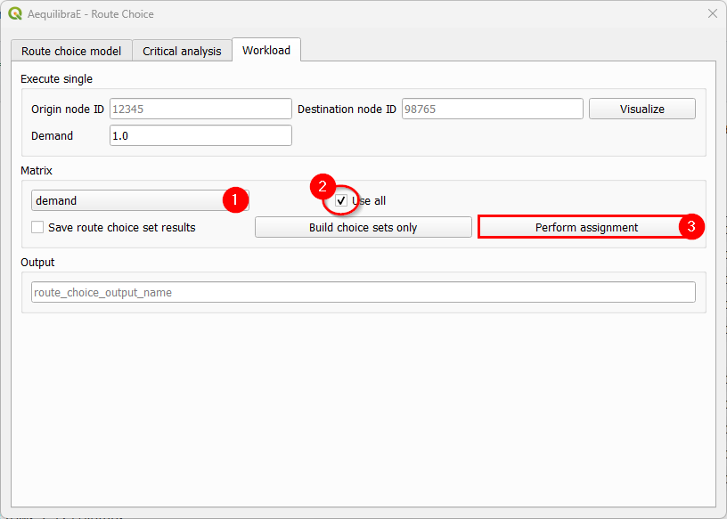
If you want to use all cores for computation, just let the “Use all” checkbox untoggled after choosing the matrix. Otherwise a table with the matrix cores and if they should be used is opened and we can select the cores we want.

Then all we need to do is hit the “Build choice sets only”. Once the task is finished, our route choice window will automatically close. If you go to the project folder, you will notice that a folder named ‘route choice’ containing folders with the choice sets for each centroid (index) in the matrix was created.

It should be noted that, although we are not performing assignment in this workflow, we use demand matrices to determine the OD pairs for which choice sets are needed, which are all of those with positive demand.

Perform assignment

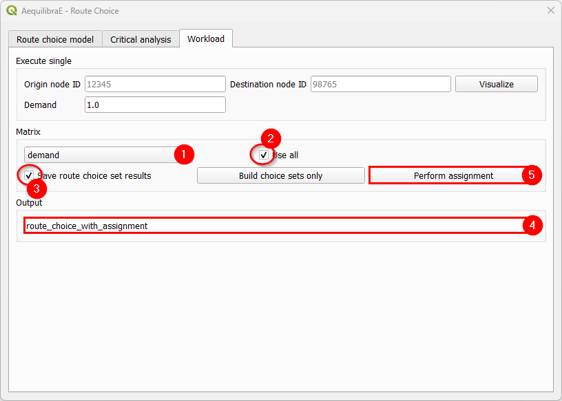
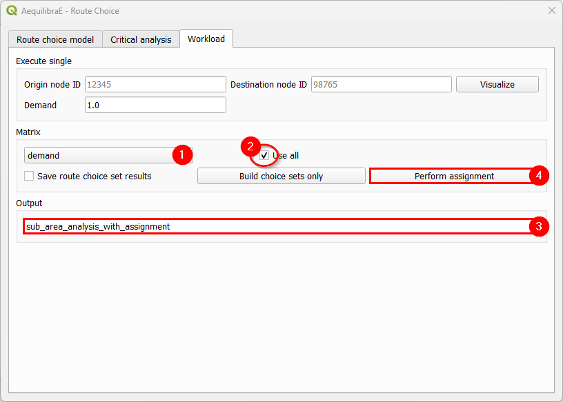
This workflow runs a route choice assignment and allows the user to save the choice set generated while performing such. The set up is quite similar to the one above: After setting the model parameters up, we go straight to the “Workload” tab and select the demand matrix and its cores for computation.

In this example, we choose to also save the choice sets generated, by toggling the “Save route choice set results” button. If we leave this button untoggled, only link flows are saved into the results database.

We also choose a name for saving the results in the database. Pick up a name that you can easily find later. Then, just hit the button “Perform assignment” and wait until the window is closed and the process is finished.

Select link analysis

The left portion of the “Critical analysis” tab gives the user access to select link analysis. Its interface is quite similar to the one in Traffic Assignment, in which we can add and remove queries with selected links, and save both the matrix and the results in the databse.

We start by toggling the “Set select link analysis” checkbox and enabling the following menus.

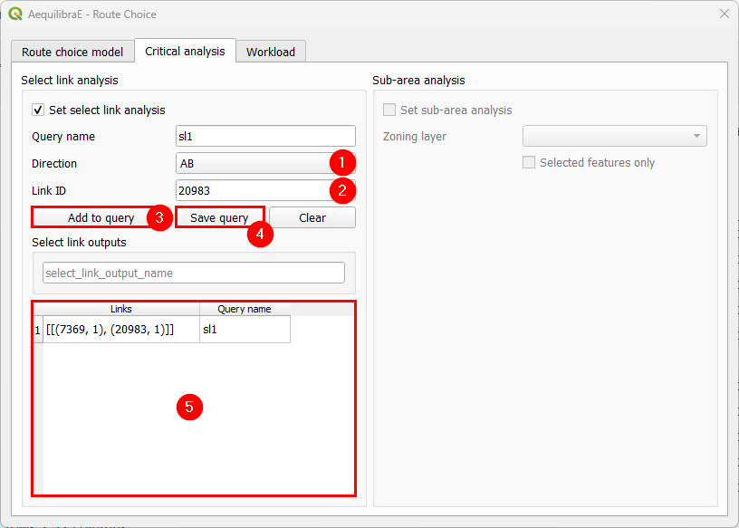
Let’s add our first query. Create a name, set the link direction, add the link ID, and click on “Add to query”.

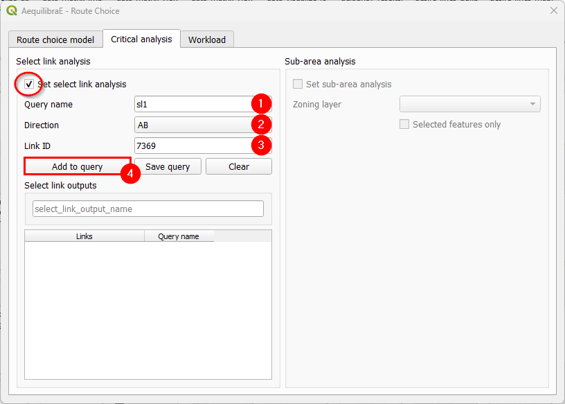
Let’s add another link to our SL1 query. Let’s set the link direction and link ID, add to the existing query with “Add to query”, and click on “Save query” (4). The SL1 query will immediately appear in the table at the bottom of the window (5).

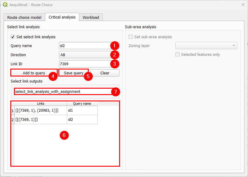
Just to make this example more interesting, let’s create an SL2 query. We repeat the process of creating a query name, setting the direction, selecting link ID, adding and saving the query. It will also appear at the bottom table (6). To remove any query from the query table, we can double-click the cell. Once this is our last query, we pick up a nice name to save our select link analysis results (7).

The last step consists in selecting the matrix and its cores for computation, and perform the assignment. It’s not necessary to add a name to the route choice output, once we did it in the previous step.

Sub-area analysis

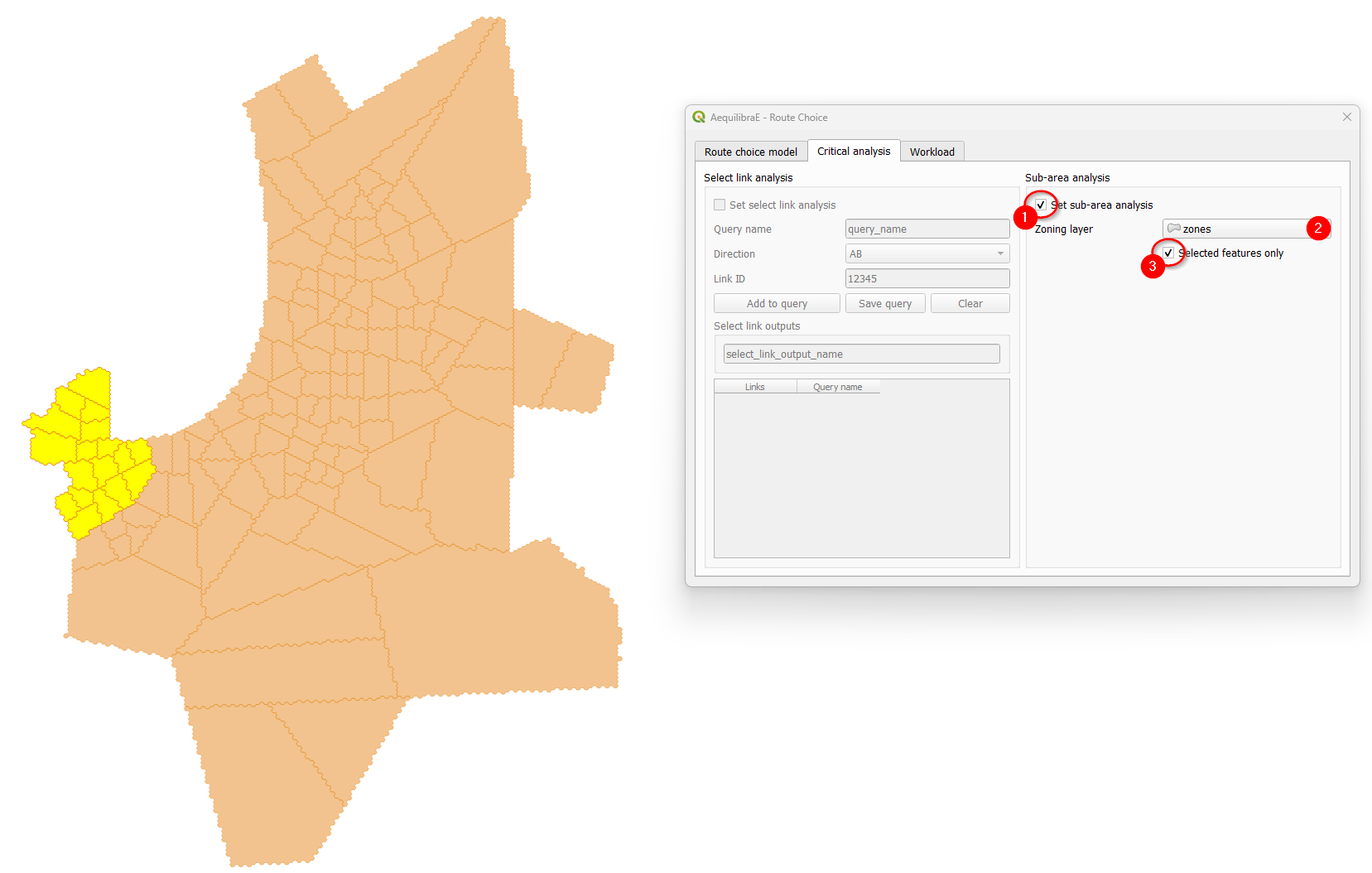
To perform a sub-area analysis, we start by toggling the “Set sub-area analysis” checkbox, which enables us to choose a polygon layer that defines the sub-area of interest. In this example, we select a couple zones in Coquimbo, and toggle the checkbox “Selected features only”. We could also use an external polygon layer with the desired region and use all the layer features rather than a part of it.

Finally, select all cores of our demand matrix for computation, don’t forget to add a name for the output file, and hit the “Perform assignment” button. When the process is finished, the window is closed. If you go to the project folder, you will notice that a folder named ‘route choice’ containing a .parquet file with the same output name you selected in (3) containing the sub-area demand matrix.

Tip

Try to reproduce AequilibraE’s Route Choice examples in QGIS!