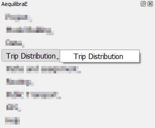
Trip Distribution

On the trip distribution tab, the user can perform Iterative Proportional Fitting (IPF) with their available matrices and vectors, as well as calibrate and apply a Synthetic Gravity Model.

In this page each option under the Trip Distribution > Trip Distribution is presented in one of the subsections below.

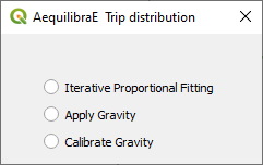
Iterative Proportional Fitting (IPF)

It is possible to balance the production/attraction vectors using IPF. There are three different ways to load a vector’s data: loading a *.csv or *.parquet file or loading data from an open layer.

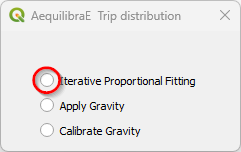
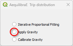
Let’s click on the Iterative Proportional Fitting option to open the menu.

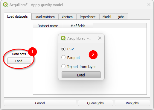
Loading the vector from a *.csv or *.parquet file is quite the same. Select your preferred option in the menu, and click Load, pointing to the location of the vector file in your machine.

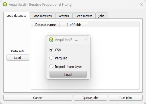
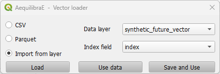
Case you are loading from an open layer, just click Import from layer, point the available data layer, and the name of its index column. You can choose between Use data or Save and use. Case you choose to save, the vector will be saved in a temporary QGIS folder.

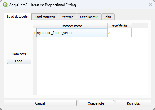
After the vector is properly loaded, it will appear in the Load datasets tab.

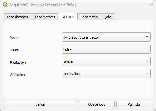
You can now select the production/attraction (origin/destination) vectors. If your data comes from a table/layer opened in QGIS, you’ll notice that the Index collapsible list is deactivated because the data index was selected when loading the data.

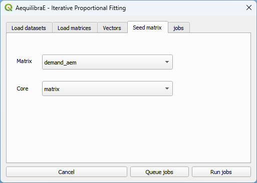
And select the impedance matrix to be used.

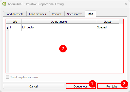
To run the procedure, simply queue the job (and select the where the output file will be saved). Then, you will notice that a job with the output file name will appear in the jobs table with a status queued (2). Finally, press Run jobs (3).

After the job is completed, a new window showing its procedure report will open.

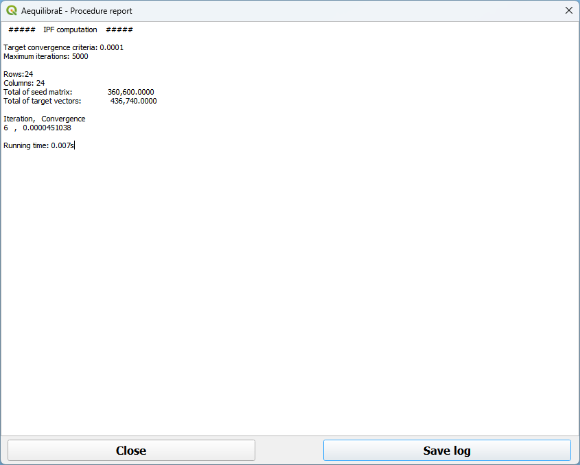
We can close it after checking the procedure report.

Important

Production and Attraction vectors must be balanced before running IPF.

Synthetic Gravity Models

Calibrate Gravity

Now that we have the demand model and a fully converged skim, we can calibrate a synthetic gravity model.

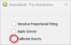
We click on Trip distribution in the AequilibraE menu and select the Calibrate Gravity model option.

The first thing to do is to check if all matrices we need (skim and demand) are in the project folder.

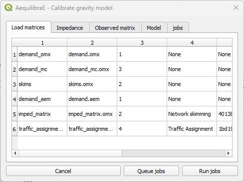
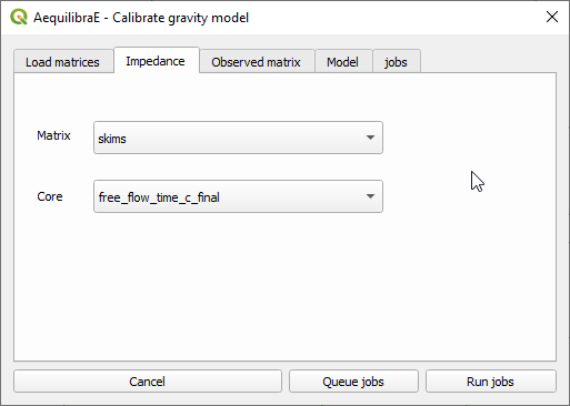
Select which matrix/matrix core is to be used as the impedance matrix.

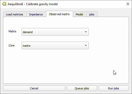
And which one corresponds to the observed matrix.

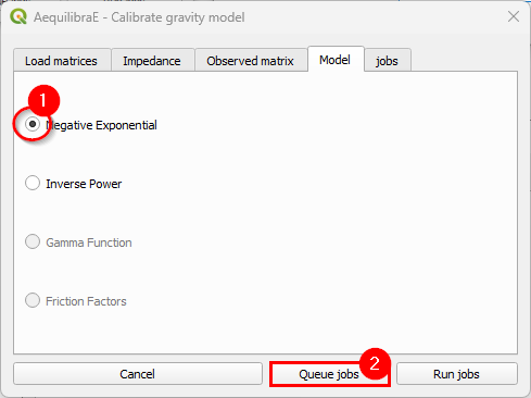
We then select which deterrence function we want to use (1) and choose a file output for the model by clicking on Queue jobs (2).

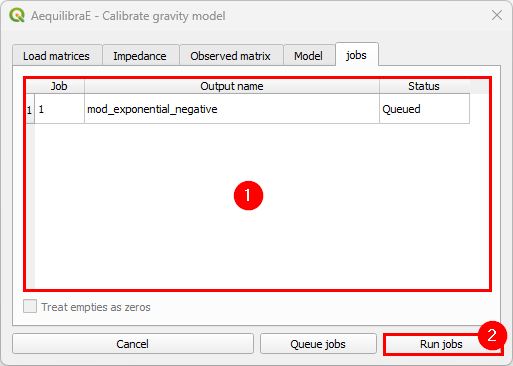
In the jobs tab, we can check all jobs we queued (1) and then run the procedure (2).

Inspect the procedure output.

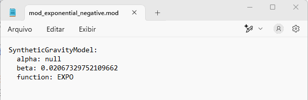
The resulting file is of type *.mod, but that is just a YAML (text file).

Apply Gravity

If one has future matrix vectors (there are some provided with the example dataset), they can either apply the Iterative Proportional Fitting (IPF) procedure available, or apply a gravity model just calibrated. Here we present the latter.

With the menu open, let’s load the dataset(s) with the production/origin and attraction/destination vectors. We can add data into the model by loading a *.csv or *.parquet file or through an open-layer, just like the IPF procedure above.

We select the production/attraction (origin/destination) vectors.

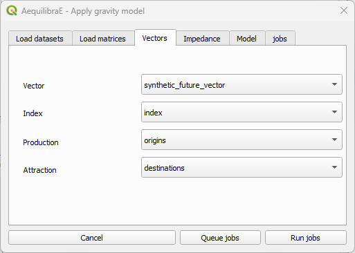
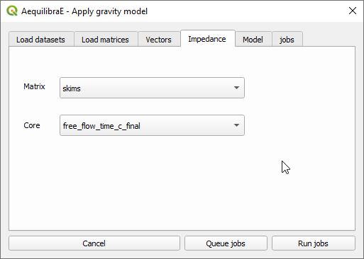
And the impedance matrix to be used. We can select one matrix core to use in computation.

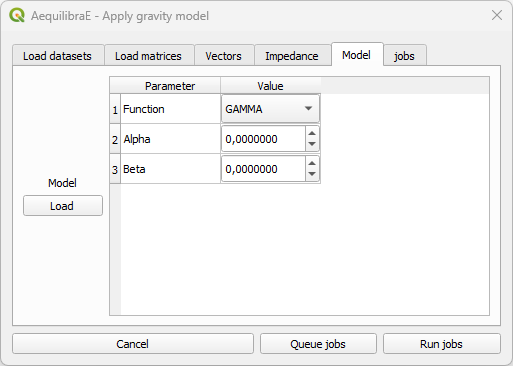
The last input is the gravity model itself, which can be done by loading a model that has been previously calibrated, or by selecting the deterrence function from the drop-down menu and typing the corresponding parameter values.

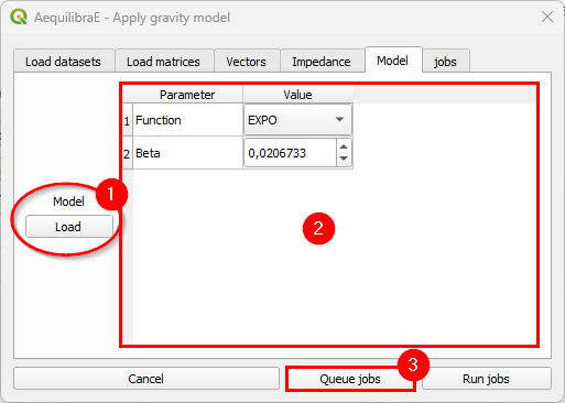
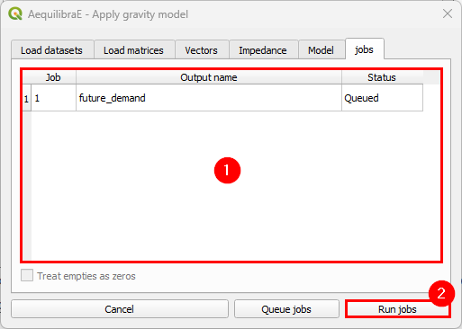
As we already have a calibrated model, we’ll load its configurations. When clicking Load (1) a new window opens. Point to the path where your *.mod file is stored, and once its done, you’ll notice that the parameters in the table view now correspond to the model data (2). Queue the jobs by hitting the Queue jobs button (3).

It is possible to check all jobs qeued before running the model in the tab Jobs (1). If all jobs look ok, just click on the Run jobs button (2).

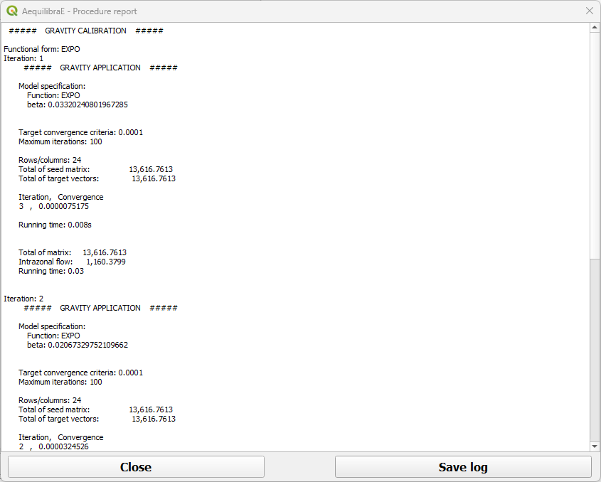
Once the process is finished, a new window with the procedure report output will open. You can check its results and then close it.

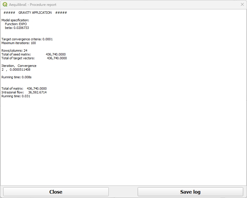
The result of this matrix can also be assigned, which is what we will generate the outputs being used in the scenario comparison.