Note
Go to the end to download the full example code.
Path computation#
In this example, we show how to perform path computation for Coquimbo, a city in La Serena Metropolitan Area in Chile.
See also
Several functions, methods, classes and modules are used in this example:
# Imports
from uuid import uuid4
from tempfile import gettempdir
from os.path import join
from aequilibrae.utils.create_example import create_example
# We create the example project inside our temp folder
fldr = join(gettempdir(), uuid4().hex)

project = create_example(fldr, "coquimbo")
import logging
import sys
We the project opens, we can tell the logger to direct all messages to the terminal as well
logger = project.logger
stdout_handler = logging.StreamHandler(sys.stdout)
formatter = logging.Formatter("%(asctime)s;%(levelname)s ; %(message)s")
stdout_handler.setFormatter(formatter)
logger.addHandler(stdout_handler)
Path Computation#
from aequilibrae.paths import PathResults
We build all graphs
project.network.build_graphs()
# We get warnings that several fields in the project are filled with ``NaN``s.
# This is true, but we won't use those fields.
2024-11-08 03:00:59,385;WARNING ; Field(s) speed, travel_time, capacity, osm_id, lanes has(ve) at least one NaN value. Check your computations
2024-11-08 03:00:59,458;WARNING ; Field(s) speed, travel_time, capacity, osm_id, lanes has(ve) at least one NaN value. Check your computations
2024-11-08 03:00:59,546;WARNING ; Field(s) speed, travel_time, capacity, osm_id, lanes has(ve) at least one NaN value. Check your computations
2024-11-08 03:00:59,632;WARNING ; Field(s) speed, travel_time, capacity, osm_id, lanes has(ve) at least one NaN value. Check your computations
We grab the graph for cars
graph = project.network.graphs["c"]

# we also see what graphs are available
project.network.graphs.keys()

# let's say we want to minimize the distance
graph.set_graph("distance")

# And will skim time and distance while we are at it
graph.set_skimming(["travel_time", "distance"])

# And we will allow paths to be computed going through other centroids/centroid connectors.
# We recommend you to `be extremely careful` with this setting.
graph.set_blocked_centroid_flows(False)
Let’s instantiate a path results object and prepare it to work with the graph
res = PathResults()
res.prepare(graph)

# compute a path from node 32343 to 22041, thats from near the airport to Fort Lambert,
# a popular location due to its views of the Coquimbo bay.
res.compute_path(32343, 22041)

# We can get the sequence of nodes we traverse
res.path_nodes
array([32343, 79778, 68225, 32487, 63937, 63192, 46510, 32380, 32373,
       55817, 55816, 11982, 46516, 75015, 79704, 79785, 78576, 68242,
       79144, 78635, 79784, 78748, 79082, 65861, 78343, 21311, 20312,
       21308, 78834, 79862, 79450, 63873, 79458, 78986, 78884, 79152,
       78645, 78549, 68503, 13380, 13383, 79199, 79745, 79457, 80001,
       78217, 78093, 80013, 25130, 80012, 40633, 11010, 11009, 40846,
       21827, 80056, 80055, 79481, 79486, 79485, 75142, 11448, 11446,
       11445, 67684, 60645, 11447, 11422, 11420, 11421, 13723, 10851,
       79462, 26681, 13718, 12079, 79460, 23707, 29778, 75451, 75445,
       45342, 39399, 13626, 13627, 45379, 21384, 63812, 40005, 12207,
       44243, 44241, 23405, 60002, 27114, 79431, 15148, 15146, 60000,
       75486, 55963, 55958, 59043, 59050, 59988, 39402, 59017, 59019,
       79398, 75520, 75516, 75512, 75509, 75505, 75511, 63544, 63543,
       75510, 75515, 75476, 63539, 30138, 11695, 61061, 30148, 44192,
       75556, 79364, 75534, 75552, 75548, 75321, 75532, 14802, 14823,
       71435, 65497, 64708, 64709, 64712, 64713, 40374, 40375, 77308,
       65518, 75566, 68526, 75573, 41306, 41308, 75619, 75617, 14899,
       14875, 38674, 75595, 65067, 65068, 79508, 29452, 44797, 29447,
       10065, 44798, 30552, 44783, 44808, 75612, 73617, 79653, 79651,
       73620, 73923, 79820, 14864, 69009, 22040, 22041])
We can get the link sequence we traverse
res.path
array([34709, 34710, 34711, 34712, 34713, 34714, 34715, 34716, 34717,
       34718, 34719, 34720, 34721, 34722,  3321,  3322,  3323,  3324,
        3325,  3326,  3327,  3328,  3329,  3330,  3331,  3332,  2970,
        2971,  2969, 19995,  1434,  1435,  1436, 19326, 19327, 19328,
       19329, 19330, 33674, 33675, 33676, 33677, 26525, 20765, 20746,
       20747, 20748, 20749, 20750, 20751, 20752,   496,   497,   498,
         499,   500,   501, 10380, 15408,   553,   552,   633,   634,
         635,   630,   631,   632,   623,   624,   625,   626,   471,
        5363, 34169, 34170, 34171, 34785,  6466,  6465, 29938, 29939,
       29940, 29941,  1446,  1447,  1448,  1449,  1450,   939,   940,
         941,  9840,  9841, 26314, 26313, 26312, 26311, 26310, 26309,
       26308, 26307, 26306, 26305, 26304, 26303, 26302, 26301, 26300,
       34079, 34147, 29962, 26422, 26421, 26420,   765,   764,   763,
         762,   761,   760,   736, 10973, 10974, 10975,   725, 10972,
         727,   728, 26424,   733,   734, 29899, 20970, 20969, 20968,
       20967, 20966, 20965, 20964, 20963, 20962,  9584,  9583, 20981,
       21398, 20982, 20983, 20984, 20985, 10030, 10031, 10032, 10033,
       10034, 10035, 10036,    64,    65, 21260, 21261, 21262, 21263,
       21264, 21265, 21266,    33, 11145, 11146,    71,    72, 34529,
       34530, 34531, 28691, 28692, 28693,  3574])
We can get the mileposts for our sequence of nodes
res.milepost
array([    0.        ,   161.94834565,   252.51996291,   390.08508135,
         549.82648658,   561.81026027,   581.36871507,   593.21987605,
         630.08836889,  1030.57121686,  1052.34444478,  1112.07906484,
        1165.81004929,  1267.22602763,  1624.43103234,  1924.50863633,
        1972.01917098,  2021.6997169 ,  2062.34315111,  2109.67655695,
        2155.98823775,  2196.91106309,  2221.69061004,  2249.01761535,
        2298.72337036,  2363.21417492,  2375.9615406 ,  2392.22488207,
        2426.81462733,  2675.27978499,  3632.15818275,  3699.27505758,
        3823.65932479,  3956.65040737,  4017.46560312,  4072.01402297,
        4129.64308736,  4163.12532905,  4187.96101397,  4224.21499938,
        4307.91646806,  4323.79479478,  4458.86701963,  4569.20833913,
        4692.25740782,  4930.34266637,  4997.45500599,  5068.23739204,
        5120.12897437,  5187.77254139,  5207.89952503,  5327.95612724,
        5368.62533167,  5378.38940327,  5385.33334293,  5426.19568418,
        5468.3231786 ,  5523.97170089,  5548.40671886,  5559.07102378,
        5592.3855075 ,  5757.7535581 ,  5923.39441593,  5950.82694781,
        5956.69374937,  5982.88386915,  6047.00805103,  6254.07203583,
        6284.94026694,  6297.98296824,  7047.68761904,  7322.48973364,
        7410.01354224,  7554.81816989,  7654.30645223,  8000.95440184,
        8009.6579379 ,  8048.90437039,  8056.1819337 ,  8230.32269321,
        8476.75016293,  8620.89727688,  9010.45521832,  9274.61196368,
        9280.12960244,  9383.74516275,  9496.88846171,  9711.90807592,
       10093.92389013, 10097.37343293, 10098.79806269, 10100.74846208,
       10158.97660612, 10308.02183308, 11038.25297634, 11043.82678472,
       11184.07536528, 11241.90536698, 11251.4005022 , 11507.50220541,
       11734.64237287, 11891.6028426 , 11914.05783947, 11931.91664218,
       11955.2823231 , 12032.22401165, 12107.39910016, 12119.5125075 ,
       12136.71574687, 12210.28469894, 12389.41094897, 12417.43348286,
       12718.35052704, 12730.00818724, 12843.38553893, 12911.9429086 ,
       12921.34664177, 13071.40008271, 13080.33320947, 13161.6119503 ,
       13335.34223859, 13388.53619865, 13412.08272452, 13574.14596808,
       13738.18613296, 13798.71647839, 14036.00947087, 14102.56840025,
       14197.10918933, 14292.09203161, 14315.76699626, 14434.43917168,
       14484.88708304, 14491.84542125, 14851.61908868, 14868.34527227,
       14877.57764797, 15028.49457611, 15037.54620347, 15204.94094821,
       15215.00009437, 15351.10413143, 15623.06737615, 15672.61684115,
       15722.54738786, 15807.97421917, 15901.71819152, 15937.27964123,
       16179.52060712, 16191.20903769, 16203.56934613, 16308.11327422,
       16479.15664668, 16536.53372128, 16548.12481843, 16559.65540426,
       16680.70266884, 16720.69837006, 16796.68692111, 16841.49843813,
       16877.97092451, 16889.16327603, 16920.08515864, 16976.52291632,
       17076.47607269, 17094.22058834, 17134.27959626, 17183.85951634,
       17472.72121764, 17554.85677394, 17659.06248146, 17923.55576674,
       17933.3892542 , 17942.66958063, 18164.10699022, 18421.89973826,
       18597.64939792, 18599.05175306])
Additionally we could also provide early_exit=True or a_star=True to compute_path
to adjust its path finding behaviour. Providing early_exit=True will allow the path finding
to quit once it’s discovered the destination, this means it will perform better for ODs that are
topographically close. However, exiting early may cause subsequent calls to update_trace
to recompute the tree in cases where it usually wouldn’t. a_star=True has precedence of early_exit=True.
res.compute_path(32343, 22041, early_exit=True)
If you’d prefer to find a potentially non-optimal path to the destination faster provide
a_star=True to use A* with a heuristic.
With this method update_trace will always recompute the path.
res.compute_path(32343, 22041, a_star=True)
By default a equirectangular heuristic is used. We can view the available heuristics via
res.get_heuristics()
['haversine', 'equirectangular']
If you’d like the more accurate, but slower, but more accurate haversine heuristic you can set it using
res.set_heuristic("haversine")
or
res.compute_path(32343, 22041, a_star=True, heuristic="haversine")
If we want to compute the path for a different destination and the same origin, we can just do this.
It is way faster when you have large networks.
Here we’ll adjust our path to the University of La Serena.
Our previous early exit and A* settings will persist with calls to update_trace.
If you’d like to adjust them for subsequent path re-computations set the res.early_exit
and res.a_star attributes.
res.a_star = False
res.update_trace(73131)
res.path_nodes
array([32343, 79778, 68225, 32487, 63937, 63192, 46510, 32380, 32373,
       55817, 55816, 11982, 46516, 75015, 79704, 79785, 78576, 68242,
       79144, 78635, 79784, 78748, 79082, 65861, 78343, 21311, 20312,
       21308, 78834, 79862, 79450, 63873, 79458, 78986, 78884, 79152,
       78645, 78549, 68503, 13380, 13383, 79199, 79745, 79457, 80001,
       78217, 78093, 80013, 25130, 80012, 40633, 11010, 11009, 40846,
       21827, 80056, 80055, 79481, 79486, 79485, 75142, 11448, 11446,
       11445, 67684, 60645, 11447, 11422, 11420, 11421, 13723, 10851,
       79462, 26681, 13718, 12079, 79460, 23707, 29778, 75451, 75445,
       45342, 39399, 13626, 13627, 45379, 21384, 63812, 40005, 12207,
       44243, 44241, 23405, 60002, 27114, 79431, 15148, 15146, 60000,
       75486, 55963, 55958, 59043, 59050, 59988, 39402, 59017, 59019,
       79398, 75520, 75516, 75512, 75509, 75505, 75511, 63544, 63543,
       75510, 75515, 75476, 63539, 30138, 11695, 61061, 30148, 44192,
       75556, 79364, 75534, 75552, 75548, 75321, 75532, 14802, 14823,
       71435, 65497, 64708, 64709, 64712, 64713, 40374, 40375, 77308,
       65518, 75566, 68526, 79517, 51754, 77189, 65059, 10093, 65058,
       30491, 66966, 66863, 30492, 77190, 77191, 79366, 77417, 79368,
       77406, 77421, 77425, 77393, 77398, 53993, 77394, 70959, 77395,
       27752, 65293, 73131])
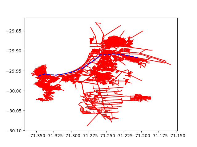
If you want to show the path in Python.
We do NOT recommend this, though… It is very slow for real networks.
import matplotlib.pyplot as plt
from shapely.ops import linemerge
links = project.network.links

# We plot the entire network
curr = project.conn.cursor()
curr.execute("Select link_id from links;")

for lid in curr.fetchall():
    geo = links.get(lid[0]).geometry
    plt.plot(*geo.xy, color="red")

path_geometry = linemerge(links.get(lid).geometry for lid in res.path)
plt.plot(*path_geometry.xy, color="blue", linestyle="dashed", linewidth=2)
plt.show()
project.close()
Total running time of the script: (1 minutes 20.792 seconds)